Chapter 5 Weakly Dependent and Stationary Time Series AR(1) Models
5.1 Efficient Market Hypothesis
We’ll test the a version of the efficient market hypothesis (EMH) by looking at weekly stock return from 1976 to 1989.
Set Time Series
/Users/Sam/Desktop/Econ 645/Data/Wooldridge

        time variable:  t, 1960w2 to 1973w16
                delta:  1 week
Our dependent variable is the weekly percentage return on the New York Stock Exchange. A strict form of the EMH states that information observable to the market prior to week t should not help to predict the return during week t. \[ E(y_t|y_{t-1},y_{t-2},...)=E(y_t) \]
We will test EMH by specifying an AR(1) model and our hypothesis states that beta for y_(t-1) will be equal to 0. We’ll assume that stock returns are serially uncorrelated, so we can safetly assume that they are weakly dependent.
\[ return_t = \beta_0 + \rho return_{t-1} + e_t \]
      Source |       SS           df       MS      Number of obs   =       689
-------------+----------------------------------   F(1, 687)       =      2.40
       Model |  10.6866231         1  10.6866231   Prob > F        =    0.1218
    Residual |  3059.73817       687  4.45376735   R-squared       =    0.0035
-------------+----------------------------------   Adj R-squared   =    0.0020
       Total |  3070.42479       688  4.46282673   Root MSE        =    2.1104

------------------------------------------------------------------------------
      return |      Coef.   Std. Err.      t    P>|t|     [95% Conf. Interval]
-------------+----------------------------------------------------------------
      return |
         L1. |   .0588984   .0380231     1.55   0.122    -.0157569    .1335538
             |
       _cons |    .179634   .0807419     2.22   0.026     .0211034    .3381646
------------------------------------------------------------------------------

      Source |       SS           df       MS      Number of obs   =       689
-------------+----------------------------------   F(1, 687)       =      2.40
       Model |  10.6866231         1  10.6866231   Prob > F        =    0.1218
    Residual |  3059.73817       687  4.45376735   R-squared       =    0.0035
-------------+----------------------------------   Adj R-squared   =    0.0020
       Total |  3070.42479       688  4.46282673   Root MSE        =    2.1104

------------------------------------------------------------------------------
      return |      Coef.   Std. Err.      t    P>|t|     [95% Conf. Interval]
-------------+----------------------------------------------------------------
    return_1 |   .0588984   .0380231     1.55   0.122    -.0157569    .1335538
       _cons |    .179634   .0807419     2.22   0.026     .0211034    .3381646
------------------------------------------------------------------------------

(2 missing values generated)

      Source |       SS           df       MS      Number of obs   =       688
-------------+----------------------------------   F(1, 687)       =      0.00
       Model |   .00603936         1   .00603936   Prob > F        =    0.9706
    Residual |  3059.08227       687  4.45281262   R-squared       =    0.0000
-------------+----------------------------------   Adj R-squared   =   -0.0015
       Total |  3059.08831       688  4.44634929   Root MSE        =    2.1102

------------------------------------------------------------------------------
           u |      Coef.   Std. Err.      t    P>|t|     [95% Conf. Interval]
-------------+----------------------------------------------------------------
           u |
         L1. |    .001405   .0381496     0.04   0.971    -.0734987    .0763087
------------------------------------------------------------------------------
We cannot reject the null hypothesis under our model, but we do have some evidence of positive serial correlation.
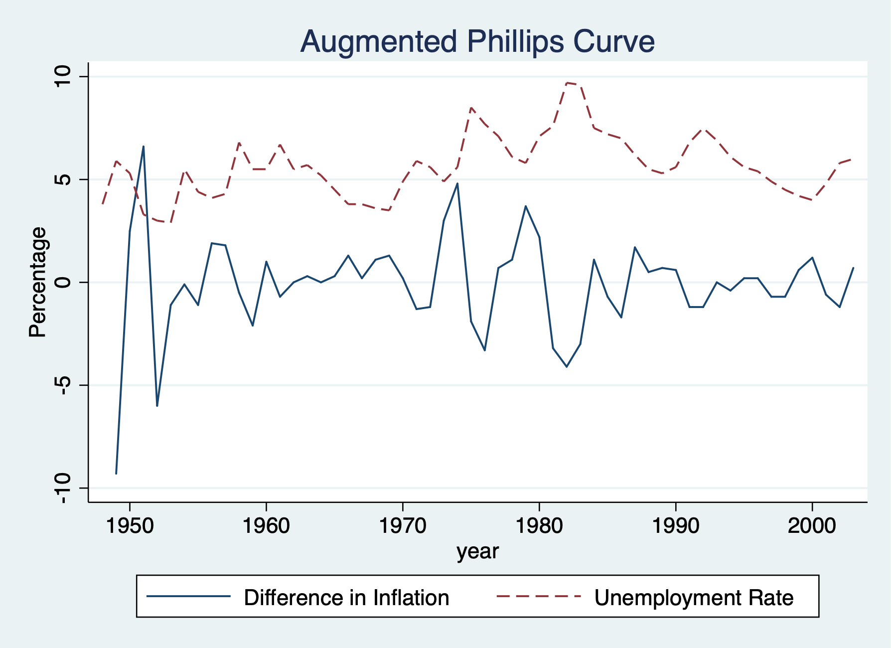
5.2 Expected Augmented Phillips Curve
We’ll revisit the Phillips curve
Set Time Series
/Users/Sam/Desktop/Econ 645/Data/Wooldridge

        time variable:  year, 1948 to 2003
                delta:  1 unit
A linear version of the expections augmented Phillips curve can be written as \[ inf_t - inf^e_t=\beta_1(unemp_t-\mu_0) + e_t \]
Where \(mu_0\) is the natural rate of unemployment and \(inf^e\) is the expected rate of inflation formed in year \(t-1\). The difference between actual unemployment and the natural rate is called cyclical unemployment, while the difference between inflation and expected inflation is called unanticipated inflation Our e_t is called our supply shock. If there is a trade-off between inflation and unemployment our \(\hat{\beta_1}\) will be negative.
An assumption is made about inflationary expectations and unders adaptive expectations, the expected value of current inflation depends on recently observed inflation. The expected inflation will be assumed to be equal to last years inflation \[ inf_t - inf_{t-1}=\beta_0 + \beta_1 unemp_t + e_t \] \[ \Delta inf_t =\beta_0 + \beta_1 unemp_t + e_t \]
Where \[ \Delta inf_t=inf_t - inf_{t-1} \] \[ \beta_0 = -\beta_1 \mu_0 \] Since \(beta_1\) is expected to be negative and \(beta_0\) is expected to be positive.
Therefore, under adaptive expectations, the augmented Phillips curve relates the change in inflation to the level of unemployment and a supply shock e_t. We’ll assume assumptions TSC.1-TSC.5 hold.
First Difference in the dependent variable or adaptive expectations of inflation.
      Source |       SS           df       MS      Number of obs   =        48
-------------+----------------------------------   F(1, 46)        =      5.56
       Model |  33.3830007         1  33.3830007   Prob > F        =    0.0227
    Residual |  276.305134        46  6.00663335   R-squared       =    0.1078
-------------+----------------------------------   Adj R-squared   =    0.0884
       Total |  309.688135        47  6.58910925   Root MSE        =    2.4508

------------------------------------------------------------------------------
        cinf |      Coef.   Std. Err.      t    P>|t|     [95% Conf. Interval]
-------------+----------------------------------------------------------------
        unem |  -.5425869   .2301559    -2.36   0.023    -1.005867    -.079307
       _cons |   3.030581    1.37681     2.20   0.033     .2592061    5.801955
------------------------------------------------------------------------------

      Source |       SS           df       MS      Number of obs   =        48
-------------+----------------------------------   F(1, 46)        =      5.56
       Model |  33.3829996         1  33.3829996   Prob > F        =    0.0227
    Residual |  276.305138        46  6.00663344   R-squared       =    0.1078
-------------+----------------------------------   Adj R-squared   =    0.0884
       Total |  309.688138        47  6.58910932   Root MSE        =    2.4508

------------------------------------------------------------------------------
       D.inf |      Coef.   Std. Err.      t    P>|t|     [95% Conf. Interval]
-------------+----------------------------------------------------------------
        unem |  -.5425869   .2301559    -2.36   0.023    -1.005867    -.079307
       _cons |   3.030581    1.37681     2.20   0.033      .259206    5.801955
------------------------------------------------------------------------------
The trade-off between unanticipated inflation and cyclical unemployment is seen in \(\hat{beta_1}\). A 1-point increase in unemployment decreases unanticipated inflation by about .54 points.
We can estimate the natural rate of unemployment by dividing \(\hat{beta_0}\) by negative of \(\hat{beta_1}\)
\[ \mu_{0} = \hat{\beta}_{0} / - \hat{\beta}_{1} \]
5.5852535Plot the graph.
twoway line cinf year || line unem year, lpattern(dash) ///
    legend(order(1 "Difference in Inflation" 2 "Unemployment Rate")) ///
    title("Augmented Phillips Curve") ytitle(Percentage) xtitle(year)

graph export "week_10_augmented_phillips.png", replace