Chapter 2 Sharp RDD
2.1 Replicate Lee, Moretti, and Butler (2004)
Lee, Moretti, and Butler (2004) wanted to test the convergence theory or the divergence theory for policy making. The convergence theory states that candidates will have to moderate their position to appeal to the median voter. The divergence theory states that the winning candidate pursues their preferred policy choices.
2.1.1 Theory
Before an election, or ex ante, voters expect a candidate to choose some policies \(x^e\) for democracts and \(y^e\) for republicans. Voters expect candidates to win with probability \(Pr(x^e,y^e)\).
When \(x^e > y^e\), then \(\frac{\partial P}{\partial x^e}>0\) and \(\frac{\partial P}{\partial y^e} < 0\).
\(P^\ast\) represents a latent (underlying but not seen) popularity of the democractic party. In other words, \(P^\ast\) is the probability that \(D\) would win if policy \(x\) is chosen at the democratic policy bliss point \(c\)
Convergence Theory: If the convergence theory holds, then \(\frac{\partial x^\ast}{\partial P^L} > 0\). An exogenuous shock in \(x^L\) would change a change in \(P^L\) and the candidate would change their position to satisfy the median voter.
Divergence Theory: If the divergence theory holds, then \(\frac{\partial x^L}{\partial P^\ast} = 0\). Popularity has no affect on policy and voters elect politicians who pursue their preferences and not the voters.
2.1.2 Potential roll-calling voting records outcomes
We are interested in potential roll-call voting records of a candidate following an election. It can be expressed in the following:
\[ RC_t=\alpha_0 + \pi_0 P^\ast_t + \pi_1 D_t + \varepsilon_t \]
Where \(RC_t\) is roll-call voting record in time period \(t\), \(P^\ast_t\) is latent popularity of the democratic party in time period \(t\), and \(D_t\) is a binary if the democratic candidate won in time period \(t\). In other words, only the winning candidate’s voting record is observed.
We are interested in potential roll-call voting records of a candidate following an election in period \(t+1\). It can be expressed in the following:
\[ RC_{t+1}=\alpha_0 + \pi_0 P^\ast_{t+1}+ \pi_1 D_{t+1} + \varepsilon_{t+1} \]
Where \(RC_{t+1}\) is roll-call voting record in time period \(t+1\), \(P^\ast_{t+1}\) is latent popularity of the democratic party in time period \(t+1\), and \(D_{t+1}\) is a binary if the democratic candidate won in time period \(t+1\).
The Problem: We never observe \(P^\ast_{t}\) and \(P^\ast_{t+1}\).
If \(D_t\) were randomized, then we could estimate an unbiased impact of _1, but we know that is not the scenario. If this holds then we have the following:
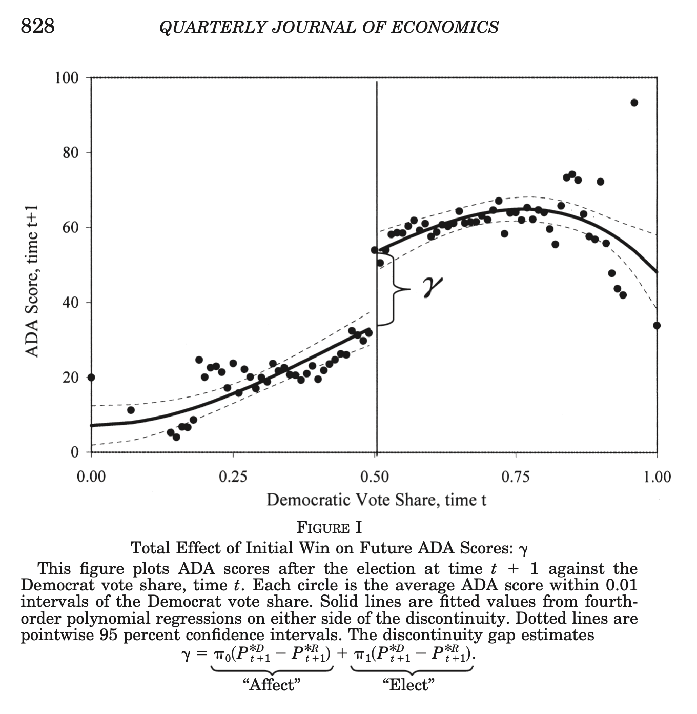
\[ \underbrace{E[RC_{t+1}|D_t=1]-E[RC_{t+1}|D_t=0]}_{Oservable} = \underbrace{\pi_0 [P^{\ast_D}_{t+1}-P^{\ast_R}_{t+1}]}_{Latent}+\underbrace{\pi_1 [P^D_{t+1}-P^R_{t+1}]}_{Observable} = \underbrace{\gamma}_{Total\ Effect} \]
Where
- \(\gamma\) is the total effect of a democratic victory in time \(t\) on future policy choice \(RC_{t+1}\)
- \(\pi_0 [P^{\ast_D}_{t+1}-P^{\ast_R}_{t+1}]\) is “Affect” component
- \(\pi_1 [P^D_{t+1}-P^R_{t+1}]\) is the “Elect” component
Key: if voters merely “elect” policies (under divergence), we should observe little change in the candidate’s intended policies following an exogenous increase in the probability in victory. Such that, the “affect” component, \(\pi_0 [P^{\ast_D}_{t+1}-P^{\ast_R}_{t+1}]\), will be very small.
What to do: Given that \(\pi_0 [P^{\ast_D}_{t+1}-P^{\ast_R}_{t+1}]\) is latent and unobservable, we will back out this part through the parts that are observable: \(\gamma\),\(\pi_1\), and \([P^D_{t+1}-P^R_{t+1}]\)
Where the elect component is composed of \(\pi_1 \ast ([P^D_{t+1}-P^R_{t+1}]\) is estimated as the difference between voting records in mean voting records between parties at time \(t\)
First, we will estimate the total effect: \(\gamma\)
\[ \underbrace{\gamma}_{Total Effect}=\underbrace{\pi_0 [P^{\ast_D}_{t+1}-P^{\ast R}_{t+1}]}_{"Affect"}+\underbrace{\pi_1 [P^{D}_{t+1}-P^{R}_{t+1}]}_{"Elect"} \]
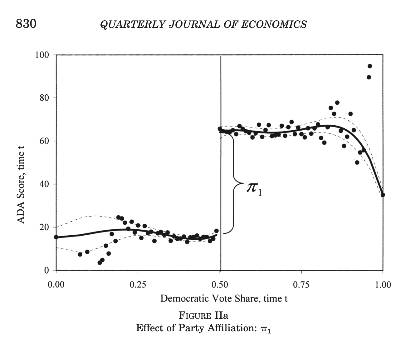
Second, we will estimate the first part of the elect component: \(\pi_1\)
\[ \underbrace{E[RC_t|D_t=1]-E[RC_t|D_t=0]}_{Observable} = \pi_1 \]
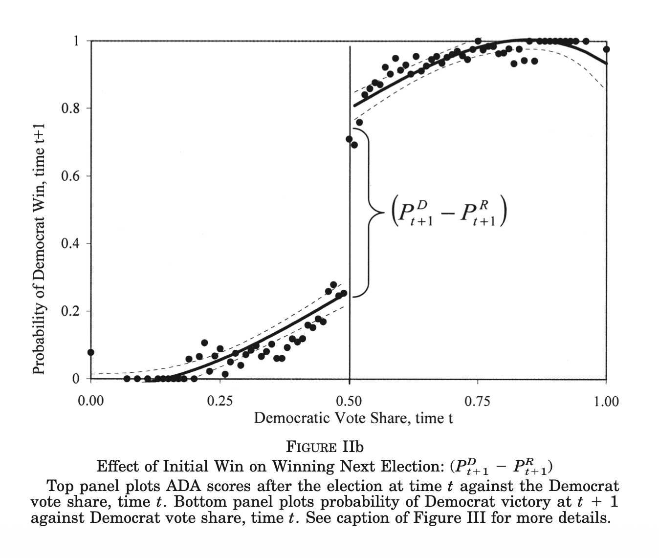
Next, we see the second part of the elect component: \(P^D_{t+1}-P^R_{t+1}\)
\[ \underbrace{E[D_{t+1}|D_t=1]-E[D_{t+1}|D_t=0]}_{Observable}=P^D_{t+1}-P^R_{t+1} \]
Next, we will use the Americans for Democractic Action (ADA) voting score that is linked to representatives in the US House of Representatives for \(RC\). The roll call is indexed from 0 to 100, where scores closer to 100 are considered more “libreral”.
We will use the vote share as the running variable.
We argue that comes from the exogenous shock in discontinuity in the running variable with a window around the cutoff
2.1.3 Replicate
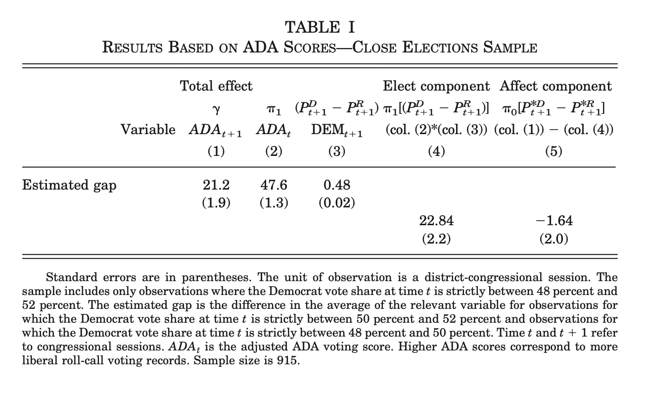
First, we will replicate Table 1 of Lee, Moretti and Butler (2004) using vote share as our running variable and 50 percent as our cutoff.
We will narrow our window to \((0.48,0.52)\) for our local regression, and cluster our errors by our \(id\) variable. Note that our \(id\) variable is state-district-year identifiers.
First we will estimate our total effect of initial win on future roll calls or \(\gamma\) using a local linear regression with a window of \([0.48,0.52]\)
use "/Users/Sam/Desktop/Econ 672/Data/lmb-data.dta", clear
reg score lagdemocrat    if lagdemvoteshare>.48 & lagdemvoteshare<.52, cluster(id)
Linear regression Number of obs = 915
F(1, 914) = 118.98
Prob > F = 0.0000
R-squared = 0.1152
Root MSE = 29.522
(Std. err. adjusted for 915 clusters in id)
------------------------------------------------------------------------------
| Robust
score | Coefficient std. err. t P>|t| [95% conf. interval]
-------------+----------------------------------------------------------------
lagdemocrat | 21.28387 1.951234 10.91 0.000 17.45445 25.11329
_cons | 31.19576 1.333983 23.39 0.000 28.57773 33.81378
------------------------------------------------------------------------------
We see a 21.28 increase in the ADA score at the discontinuity, which includes the “elect” and “affect” components.
Next, we will estimate \(\pi_1\) from the elect component using a local regression using a window of \([0.48,0.52]\).
Linear regression                               Number of obs     =        915
                                                F(1, 914)         =    1237.69
                                                Prob > F          =     0.0000
                                                R-squared         =     0.5783
                                                Root MSE          =      20.38

                                   (Std. err. adjusted for 915 clusters in id)
------------------------------------------------------------------------------
             |               Robust
       score | Coefficient  std. err.      t    P>|t|     [95% conf. interval]
-------------+----------------------------------------------------------------
    democrat |    47.7056   1.356011    35.18   0.000     45.04434    50.36686
       _cons |    18.7469   .8432428    22.23   0.000     17.09198    20.40182
------------------------------------------------------------------------------
Our \(\hat{\pi}_1\) is 47.6, which is the increase in ADA scores at time \(t\) due to a \(D\) treatment/win.
Next, we will calculate \(P^D_{t+1} - P^R_{t+1}\)
Linear regression                               Number of obs     =        915
                                                F(1, 914)         =     280.23
                                                Prob > F          =     0.0000
                                                R-squared         =     0.2348
                                                Root MSE          =     .43767

                                   (Std. err. adjusted for 915 clusters in id)
------------------------------------------------------------------------------
             |               Robust
    democrat | Coefficient  std. err.      t    P>|t|     [95% conf. interval]
-------------+----------------------------------------------------------------
 lagdemocrat |   .4843287   .0289322    16.74   0.000     .4275475    .5411099
       _cons |   .2417582   .0200939    12.03   0.000     .2023227    .2811938
------------------------------------------------------------------------------
Our \(\hat{\pi}_1 * \widehat{(PDt+1 - PRt+1)}\) is 0.48, which is the effect of initial win on winning the next election.
Now, we have all three of our estimate, so we can back out the “affect” component.
\[ \widehat{\gamma} - (\hat{\pi}_1 * \widehat{(PDt+1 - PRt+1)}) = \hat{\pi}_0 \] The gap at 0.5 comes from \(\pi_1\) or “elect” and not \(\pi_0\) or “affect”.
We can see this in the authors’ results.
2.2 Different functional forms of RDD
Now we will replicate Lee, et al. (2004) using different specifications for the RDD. First, we will use all of the data with OLS instead of a local regression without a running variable. Next, we will incorporate a recentered running variable using all of the data. Then, we will use an interaction term between treatment and the running variable using all of the data. For our last global regression, we will use a quadratic interaction term between our running variable and the treatment. Finally, we will use a local regression.
2.2.1 Treatment with no running variable
We will use all of the data instead of just the window around the cutoff. This is the full data set and not a local linear regression.
reg score lagdemocrat, cluster(id)
reg score democrat, cluster(id)
reg democrat lagdemocrat, cluster(id)
Linear regression Number of obs = 13,588
F(1, 13587) = 4243.29
Prob > F = 0.0000
R-squared = 0.2267
Root MSE = 28.694
(Std. err. adjusted for 13,588 clusters in id)
------------------------------------------------------------------------------
| Robust
score | Coefficient std. err. t P>|t| [95% conf. interval]
-------------+----------------------------------------------------------------
lagdemocrat | 31.50628 .483666 65.14 0.000 30.55823 32.45433
_cons | 23.53946 .3374569 69.76 0.000 22.87799 24.20092
------------------------------------------------------------------------------
Linear regression Number of obs = 13,588
F(1, 13587) = 9502.26
Prob > F = 0.0000
R-squared = 0.3756
Root MSE = 25.785
(Std. err. adjusted for 13,588 clusters in id)
------------------------------------------------------------------------------
| Robust
score | Coefficient std. err. t P>|t| [95% conf. interval]
-------------+----------------------------------------------------------------
democrat | 40.76266 .4181664 97.48 0.000 39.94299 41.58232
_cons | 17.5756 .2625459 66.94 0.000 17.06097 18.09022
------------------------------------------------------------------------------
Linear regression Number of obs = 13,588
F(1, 13587) = 25739.79
Prob > F = 0.0000
R-squared = 0.6759
Root MSE = .27929
(Std. err. adjusted for 13,588 clusters in id)
------------------------------------------------------------------------------
| Robust
democrat | Coefficient std. err. t P>|t| [95% conf. interval]
-------------+----------------------------------------------------------------
lagdemocrat | .8178836 .0050979 160.44 0.000 .807891 .8278761
_cons | .1201058 .0043176 27.82 0.000 .1116428 .1285688
------------------------------------------------------------------------------We can see that our discontinuities are qiuet different under a global regression. However, we do not control the running variable, so we should not put too much stock in these results.
Note: Stata code attributed to Marcelo Perraillon.
2.2.2 Recentered running variable and treatment
Next, we will recenter our running variable and use a global regression. We recenter our 0 to 1 vote share by subtracting by 0.5. So our range becomes \([-0.5,0.5]\) with 0 being our center.
Recenter running variable of voteshare and rerun regressions
gen demvoteshare_c = demvoteshare - 0.5
reg score lagdemocrat demvoteshare_c, cluster(id)
reg score democrat demvoteshare_c, cluster(id)
reg democrat lagdemocrat demvoteshare_c, cluster(id)
(11 missing values generated)
Linear regression Number of obs = 13,577
F(2, 13576) = 2115.71
Prob > F = 0.0000
R-squared = 0.2274
Root MSE = 28.686
(Std. err. adjusted for 13,577 clusters in id)
--------------------------------------------------------------------------------
| Robust
score | Coefficient std. err. t P>|t| [95% conf. interval]
---------------+----------------------------------------------------------------
lagdemocrat | 33.45118 .8481987 39.44 0.000 31.7886 35.11377
demvoteshare_c | -5.62558 1.898081 -2.96 0.003 -9.346082 -1.905077
_cons | 22.88345 .4433244 51.62 0.000 22.01447 23.75242
--------------------------------------------------------------------------------
Linear regression Number of obs = 13,577
F(2, 13576) = 6192.13
Prob > F = 0.0000
R-squared = 0.4242
Root MSE = 24.764
(Std. err. adjusted for 13,577 clusters in id)
--------------------------------------------------------------------------------
| Robust
score | Coefficient std. err. t P>|t| [95% conf. interval]
---------------+----------------------------------------------------------------
democrat | 58.50236 .65638 89.13 0.000 57.21576 59.78895
demvoteshare_c | -48.93761 1.641489 -29.81 0.000 -52.15516 -45.72006
_cons | 11.03413 .3363049 32.81 0.000 10.37493 11.69334
--------------------------------------------------------------------------------
Linear regression Number of obs = 13,577
F(2, 13576) = 48967.17
Prob > F = 0.0000
R-squared = 0.7354
Root MSE = .25242
(Std. err. adjusted for 13,577 clusters in id)
--------------------------------------------------------------------------------
| Robust
democrat | Coefficient std. err. t P>|t| [95% conf. interval]
---------------+----------------------------------------------------------------
lagdemocrat | .5516115 .0103234 53.43 0.000 .5313761 .5718469
demvoteshare_c | .7725248 .0187564 41.19 0.000 .7357597 .8092898
_cons | .2116664 .0052743 40.13 0.000 .2013279 .2220048
--------------------------------------------------------------------------------Our results are closer to Lee, et al. (2004), but they are still far off. Please note that we keep the function form of the slope for the running variable the same on both sides of the cutoff.
Note: Stata code attributed to Marcelo Perraillon.
2.2.3 Interaction between treatment and running variable
We are going to allow for intercepts and slopes to differ with interacting categorical and continuous variables. Why do we want to do this? We allow for the slope to differ on both sides of the discontinuity. As seen above in Figure 1, the slopes may differ on each side of the discontinuity.
Please note that Cunningham likes to use the xi:, while I prefer to use the interaction operators ##.
xi: reg score i.lagdemocrat*demvoteshare_c, cluster(id)
xi: reg score i.democrat*demvoteshare_c, cluster(id)
xi: reg democrat i.lagdemocrat*demvoteshare_c, cluster(id)
i.lagdemocrat _Ilagdemocr_0-1 (naturally coded; _Ilagdemocr_0 omitted)
i.lagd~t*demv~c _IlagXdemvo_# (coded as above)
Linear regression Number of obs = 13,577
F(3, 13576) = 1863.06
Prob > F = 0.0000
R-squared = 0.2669
Root MSE = 27.944
(Std. err. adjusted for 13,577 clusters in id)
--------------------------------------------------------------------------------
| Robust
score | Coefficient std. err. t P>|t| [95% conf. interval]
---------------+----------------------------------------------------------------
_Ilagdemocr_1 | 30.50803 .8172343 37.33 0.000 28.90614 32.10993
demvoteshare_c | 66.04181 3.159572 20.90 0.000 59.84861 72.23501
_IlagXdemvo_1 | -96.47474 3.851734 -25.05 0.000 -104.0247 -88.92481
_cons | 31.43518 .5409599 58.11 0.000 30.37482 32.49554
--------------------------------------------------------------------------------
i.democrat _Idemocrat_0-1 (naturally coded; _Idemocrat_0 omitted)
i.demo~t*demv~c _IdemXdemvo_# (coded as above)
Linear regression Number of obs = 13,577
F(3, 13576) = 4160.73
Prob > F = 0.0000
R-squared = 0.4344
Root MSE = 24.544
(Std. err. adjusted for 13,577 clusters in id)
--------------------------------------------------------------------------------
| Robust
score | Coefficient std. err. t P>|t| [95% conf. interval]
---------------+----------------------------------------------------------------
_Idemocrat_1 | 55.43136 .6373768 86.97 0.000 54.18201 56.68071
demvoteshare_c | -5.682785 2.609124 -2.18 0.029 -10.79703 -.5685407
_IdemXdemvo_1 | -55.15188 3.217652 -17.14 0.000 -61.45893 -48.84484
_cons | 16.81598 .4184826 40.18 0.000 15.9957 17.63627
--------------------------------------------------------------------------------
i.lagdemocrat _Ilagdemocr_0-1 (naturally coded; _Ilagdemocr_0 omitted)
i.lagd~t*demv~c _IlagXdemvo_# (coded as above)
Linear regression Number of obs = 13,577
F(3, 13576) = 25212.81
Prob > F = 0.0000
R-squared = 0.7489
Root MSE = .2459
(Std. err. adjusted for 13,577 clusters in id)
--------------------------------------------------------------------------------
| Robust
democrat | Coefficient std. err. t P>|t| [95% conf. interval]
---------------+----------------------------------------------------------------
_Ilagdemocr_1 | .5257231 .0104514 50.30 0.000 .505237 .5462092
demvoteshare_c | 1.402922 .0443487 31.63 0.000 1.315993 1.489852
_IlagXdemvo_1 | -.8486068 .0490015 -17.32 0.000 -.9446565 -.7525571
_cons | .2868887 .0077506 37.02 0.000 .2716965 .3020809
--------------------------------------------------------------------------------Note: xi is interaction expansion: https://www.stata.com/manuals13/rxi.pdf
Note: Stata code attributed to Marcelo Perraillon.
You can use ## between to variables for interactions as well (I prefer this method). You use i.varname for the categorical and c.varname for the continuous. So we are interacting a binary variable with a continuous one here to allow for different slopes and intercepts.
reg score i.lagdemocrat##c.demvoteshare_c, cluster(id)
reg score i.democrat##c.demvoteshare_c, cluster(id)
reg democrat i.lagdemocrat##c.demvoteshare_c, cluster(id)
Linear regression Number of obs = 13,577
F(3, 13576) = 1863.06
Prob > F = 0.0000
R-squared = 0.2669
Root MSE = 27.944
(Std. err. adjusted for 13,577 clusters in id)
--------------------------------------------------------------------------------
| Robust
score | Coefficient std. err. t P>|t| [95% conf. interval]
---------------+----------------------------------------------------------------
1.lagdemocrat | 30.50803 .8172343 37.33 0.000 28.90614 32.10993
demvoteshare_c | 66.04181 3.159572 20.90 0.000 59.84861 72.23501
|
lagdemocrat#|
c. |
demvoteshare_c |
1 | -96.47474 3.851734 -25.05 0.000 -104.0247 -88.92481
|
_cons | 31.43518 .5409599 58.11 0.000 30.37482 32.49554
--------------------------------------------------------------------------------
Linear regression Number of obs = 13,577
F(3, 13576) = 4160.73
Prob > F = 0.0000
R-squared = 0.4344
Root MSE = 24.544
(Std. err. adjusted for 13,577 clusters in id)
--------------------------------------------------------------------------------
| Robust
score | Coefficient std. err. t P>|t| [95% conf. interval]
---------------+----------------------------------------------------------------
1.democrat | 55.43136 .6373768 86.97 0.000 54.18201 56.68071
demvoteshare_c | -5.682785 2.609124 -2.18 0.029 -10.79703 -.5685407
|
democrat#|
c. |
demvoteshare_c |
1 | -55.15188 3.217652 -17.14 0.000 -61.45893 -48.84484
|
_cons | 16.81598 .4184826 40.18 0.000 15.9957 17.63627
--------------------------------------------------------------------------------
Linear regression Number of obs = 13,577
F(3, 13576) = 25212.81
Prob > F = 0.0000
R-squared = 0.7489
Root MSE = .2459
(Std. err. adjusted for 13,577 clusters in id)
--------------------------------------------------------------------------------
| Robust
democrat | Coefficient std. err. t P>|t| [95% conf. interval]
---------------+----------------------------------------------------------------
1.lagdemocrat | .5257231 .0104514 50.30 0.000 .505237 .5462092
demvoteshare_c | 1.402922 .0443487 31.63 0.000 1.315993 1.489852
|
lagdemocrat#|
c. |
demvoteshare_c |
1 | -.8486068 .0490015 -17.32 0.000 -.9446565 -.7525571
|
_cons | .2868887 .0077506 37.02 0.000 .2716965 .3020809
--------------------------------------------------------------------------------With our full-sample interaction, we are starting to get closer to our results from the local linear regression and the results Lee, Moretti, and Butler (2004).
2.2.4 Quadratic interaction between treatment and running variable
Next, we will use a global linear regression using an quadratic interaction. Why do we want to use a quadratic interaction? Not only do we allow the slopes to differ, we also allow for flexibility in the function form. This will better match the data on both sides of the discontinuity. Furthermore, if we misspecify the functinoal form, then we may attribute a discontinuity when one does not exist.
gen demvoteshare_sq = demvoteshare_c^2
reg score i.lagdemocrat##c.(demvoteshare_c demvoteshare_sq), cluster(id)
reg score i.democrat##c.(demvoteshare_c demvoteshare_sq), cluster(id)
reg democrat i.lagdemocrat##c.(demvoteshare_c demvoteshare_sq), cluster(id)
Linear regression Number of obs = 13,577
F(5, 13576) = 1529.38
Prob > F = 0.0000
R-squared = 0.3707
Root MSE = 25.892
(Std. err. adjusted for 13,577 clusters in id)
---------------------------------------------------------------------------------
| Robust
score | Coefficient std. err. t P>|t| [95% conf. interval]
----------------+----------------------------------------------------------------
1.lagdemocrat | 13.02968 1.268439 10.27 0.000 10.54337 15.516
demvoteshare_c | 134.9765 9.634337 14.01 0.000 116.0919 153.8611
demvoteshare_sq | 212.1269 22.39469 9.47 0.000 168.2302 256.0236
|
lagdemocrat#|
c. |
demvoteshare_c |
1 | 57.05469 15.15178 3.77 0.000 27.35509 86.7543
|
lagdemocrat#|
c. |
demvoteshare_sq |
1 | -641.8509 30.80241 -20.84 0.000 -702.2279 -581.4739
|
_cons | 33.54745 .7068697 47.46 0.000 32.16189 34.93302
---------------------------------------------------------------------------------
Linear regression Number of obs = 13,577
F(5, 13576) = 2589.02
Prob > F = 0.0000
R-squared = 0.4559
Root MSE = 24.075
(Std. err. adjusted for 13,577 clusters in id)
---------------------------------------------------------------------------------
| Robust
score | Coefficient std. err. t P>|t| [95% conf. interval]
----------------+----------------------------------------------------------------
1.democrat | 44.40229 .9086222 48.87 0.000 42.62126 46.18331
demvoteshare_c | -23.8496 6.710943 -3.55 0.000 -37.00398 -10.69522
demvoteshare_sq | -41.72917 14.67192 -2.84 0.004 -70.48817 -12.97018
|
democrat#|
c. |
demvoteshare_c |
1 | 111.8963 9.779383 11.44 0.000 92.72733 131.0652
|
democrat#|
c. |
demvoteshare_sq |
1 | -229.9544 19.53577 -11.77 0.000 -268.2472 -191.6615
|
_cons | 15.60635 .5747061 27.16 0.000 14.47984 16.73285
---------------------------------------------------------------------------------
Linear regression Number of obs = 13,577
F(5, 13576) = 89733.30
Prob > F = 0.0000
R-squared = 0.8220
Root MSE = .20703
(Std. err. adjusted for 13,577 clusters in id)
---------------------------------------------------------------------------------
| Robust
democrat | Coefficient std. err. t P>|t| [95% conf. interval]
----------------+----------------------------------------------------------------
1.lagdemocrat | .3216837 .0181913 17.68 0.000 .2860263 .3573411
demvoteshare_c | 2.798344 .1928588 14.51 0.000 2.420314 3.176374
demvoteshare_sq | 4.294014 .4472409 9.60 0.000 3.41736 5.170668
|
lagdemocrat#|
c. |
demvoteshare_c |
1 | .0909402 .2371611 0.38 0.701 -.3739284 .5558089
|
lagdemocrat#|
c. |
demvoteshare_sq |
1 | -8.804368 .5077003 -17.34 0.000 -9.799531 -7.809205
|
_cons | .3296468 .0125535 26.26 0.000 .3050402 .3542534
---------------------------------------------------------------------------------With our quadratic interaction, we start to move away from our local linear regression (except for the estimate of \(\pi_1\)). Our estimates of \(\gamma\) and \((PDt+1 - PRt+1)\) are far off from where we expect them to be.
2.2.5 Local regression: 5 points from cutoff with OLS
Finally, we will use a local linear regression with a quadratic interaction. With our local linear regression with a quadratic interaction, we narrow our window, but we allow for a more flexible functional form on both sides of the discontinuity.
reg score i.lagdemocrat##c.(demvoteshare_c demvoteshare_sq) if lagdemvoteshare>.45 & lagdemvoteshare<.55, cluster(id)
reg score i.democrat##c.(demvoteshare_c demvoteshare_sq) if lagdemvoteshare>.45 & lagdemvoteshare<.55, cluster(id)
reg democrat i.lagdemocrat##c.(demvoteshare_c demvoteshare_sq) if lagdemvoteshare>.45 & lagdemvoteshare<.55, cluster(id)
Linear regression Number of obs = 2,441
F(5, 2440) = 261.93
Prob > F = 0.0000
R-squared = 0.4048
Root MSE = 23.951
(Std. err. adjusted for 2,441 clusters in id)
---------------------------------------------------------------------------------
| Robust
score | Coefficient std. err. t P>|t| [95% conf. interval]
----------------+----------------------------------------------------------------
1.lagdemocrat | 3.967238 1.490509 2.66 0.008 1.044445 6.890032
demvoteshare_c | 241.8926 20.54643 11.77 0.000 201.6023 282.1828
demvoteshare_sq | 407.0713 62.42092 6.52 0.000 284.6678 529.4748
|
lagdemocrat#|
c. |
demvoteshare_c |
1 | 27.51541 28.75342 0.96 0.339 -28.86823 83.89905
|
lagdemocrat#|
c. |
demvoteshare_sq |
1 | -1002.938 79.32636 -12.64 0.000 -1158.492 -847.3844
|
_cons | 40.65686 .9475232 42.91 0.000 38.79883 42.51489
---------------------------------------------------------------------------------
Linear regression Number of obs = 2,441
F(5, 2440) = 717.83
Prob > F = 0.0000
R-squared = 0.5801
Root MSE = 20.117
(Std. err. adjusted for 2,441 clusters in id)
---------------------------------------------------------------------------------
| Robust
score | Coefficient std. err. t P>|t| [95% conf. interval]
----------------+----------------------------------------------------------------
1.democrat | 46.87991 1.542781 30.39 0.000 43.85462 49.90521
demvoteshare_c | -27.71422 15.03124 -1.84 0.065 -57.18953 1.761092
demvoteshare_sq | -87.87141 29.14324 -3.02 0.003 -145.0195 -30.72336
|
democrat#|
c. |
demvoteshare_c |
1 | 78.48126 23.09883 3.40 0.001 33.18592 123.7766
|
democrat#|
c. |
demvoteshare_sq |
1 | -132.0792 50.97886 -2.59 0.010 -232.0455 -32.11286
|
_cons | 17.51743 1.013373 17.29 0.000 15.53027 19.50459
---------------------------------------------------------------------------------
Linear regression Number of obs = 2,441
F(5, 2440) = 1642.94
Prob > F = 0.0000
R-squared = 0.7005
Root MSE = .27372
(Std. err. adjusted for 2,441 clusters in id)
---------------------------------------------------------------------------------
| Robust
democrat | Coefficient std. err. t P>|t| [95% conf. interval]
----------------+----------------------------------------------------------------
1.lagdemocrat | .1181676 .0203498 5.81 0.000 .0782629 .1580723
demvoteshare_c | 5.095347 .3027069 16.83 0.000 4.501758 5.688936
demvoteshare_sq | 9.265549 .9176752 10.10 0.000 7.466046 11.06505
|
lagdemocrat#|
c. |
demvoteshare_c |
1 | .0359484 .38651 0.09 0.926 -.7219732 .79387
|
lagdemocrat#|
c. |
demvoteshare_sq |
1 | -18.30185 1.05566 -17.34 0.000 -20.37193 -16.23176
|
_cons | .4411991 .0135581 32.54 0.000 .4146126 .4677855
---------------------------------------------------------------------------------Interestingly, our local linear regression with a quadratic interaction does much worse for estimating \(\gamma\) and \((PDt+1 - PRt+1)\)