Chapter 1 Propensity Score Matching
We will go through the process of manually estimating propensity scores before we use the teffects commands. After estimating the propensity scores, we will estimate the \(ATE\) and \(ATT\)
We will use the data from Dehejia and Wahba (2002) for treatment from Department of Labor Employment and Training Adminstration (ETA) job training. Instead of using the control group from the orgininal RCT, we will use data from the Current Population Survey (CPS) for a comparison group.
1.1 Generate propensity score
First, we will import and drop the experimental control group, so we can append our comparison group from the CPS.
Now merge in the CPS controls from footnote 2 of Table 2 (Dehejia and Wahba 2002)
Now we will generate additional variables of interest: age, education, demographics, and unemployment status
gen agesq=age*age
gen agecube=age*age*age
gen edusq=educ*edu
gen u74 = 0 if re74!=.
replace u74 = 1 if re74==0
gen u75 = 0 if re75!=.
replace u75 = 1 if re75==0
gen interaction1 = educ*re74
gen re74sq=re74^2
gen re75sq=re75^2
gen interaction2 = u74*hisp
Next, we will use logistic regression to estimate \(\beta\) and estimate the \(p\)-scores.
logit treat age agesq agecube educ edusq marr nodegree black hisp re74 re75 u74 u75 interaction1
predict pscore
Iteration 0: Log likelihood = -1011.0713
Iteration 1: Log likelihood = -612.55814
Iteration 2: Log likelihood = -429.05652
Iteration 3: Log likelihood = -406.25926
Iteration 4: Log likelihood = -404.18813
Iteration 5: Log likelihood = -404.15991
Iteration 6: Log likelihood = -404.15991
Logistic regression Number of obs = 16,177
LR chi2(14) = 1213.82
Prob > chi2 = 0.0000
Log likelihood = -404.15991 Pseudo R2 = 0.6003
------------------------------------------------------------------------------
treat | Coefficient Std. err. z P>|z| [95% conf. interval]
-------------+----------------------------------------------------------------
age | 2.425229 .3500651 6.93 0.000 1.739114 3.111344
agesq | -.0672395 .0111308 -6.04 0.000 -.0890555 -.0454234
agecube | .0005685 .0001113 5.11 0.000 .0003505 .0007866
educ | .9247847 .2500694 3.70 0.000 .4346576 1.414912
edusq | -.0572021 .0136202 -4.20 0.000 -.0838972 -.030507
marr | -1.556471 .2517687 -6.18 0.000 -2.049929 -1.063013
nodegree | .9270591 .3254621 2.85 0.004 .2891651 1.564953
black | 3.850668 .2662868 14.46 0.000 3.328755 4.37258
hisp | 1.673885 .4099129 4.08 0.000 .8704704 2.4773
re74 | -.0002203 .0001086 -2.03 0.043 -.0004332 -7.40e-06
re75 | -.0001969 .0000378 -5.21 0.000 -.000271 -.0001228
u74 | 1.749522 .2897311 6.04 0.000 1.18166 2.317385
u75 | .00944 .257531 0.04 0.971 -.4953114 .5141915
interaction1 | .0000222 9.08e-06 2.45 0.014 4.43e-06 .00004
_cons | -35.22098 3.797922 -9.27 0.000 -42.66477 -27.77719
------------------------------------------------------------------------------
Note: 3 failures and 0 successes completely determined.
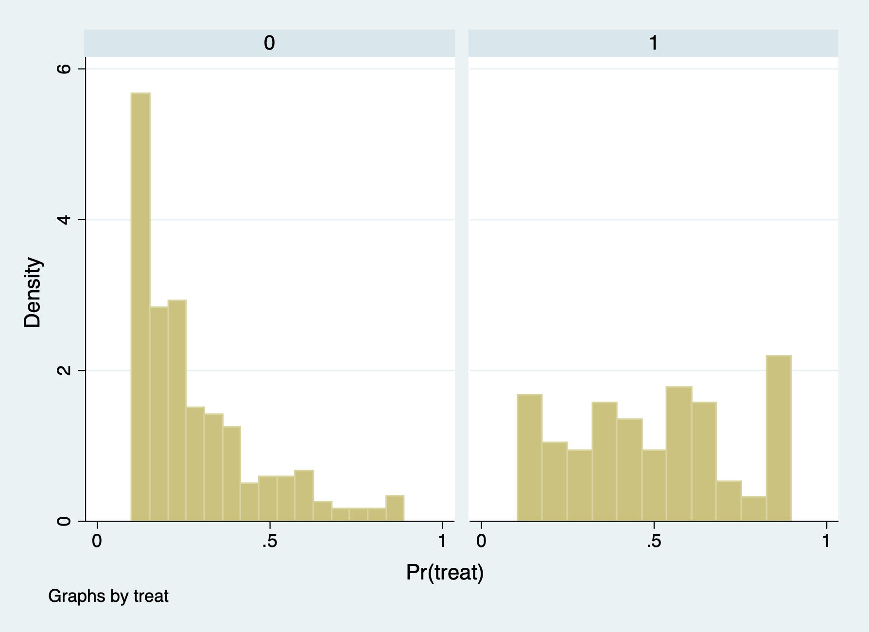
(option pr assumed; Pr(treat))Now, we will compare the propensity score between treatment and comparison groups with summary statistics and histograms.
                          Pr(treat)
-------------------------------------------------------------
      Percentiles      Smallest
 1%     .0011757       .0010614
 5%     .0072641       .0011757
10%     .0260147       .0018463       Obs                 185
25%     .1322174       .0020981       Sum of wgt.         185

50%     .4001992                      Mean           .4253567
                        Largest       Std. dev.      .3076908
75%     .6706164        .935645
90%     .8866026         .93718       Variance       .0946736
95%     .9021386       .9374608       Skewness       .1916478
99%     .9374608       .9384554       Kurtosis       1.732134

                          Pr(treat)
-------------------------------------------------------------
      Percentiles      Smallest
 1%     5.90e-07       1.18e-09
 5%     1.72e-06       4.07e-09
10%     3.58e-06       4.24e-09       Obs              15,992
25%     .0000193       1.55e-08       Sum of wgt.      15,992

50%     .0001187                      Mean           .0066476
                        Largest       Std. dev.      .0416672
75%     .0009635       .8786677
90%     .0066319       .8893389       Variance       .0017362
95%     .0163109       .9099022       Skewness        12.2493
99%     .1551548       .9239787       Kurtosis       187.8692
The comparison group has a mean propensity score of 0.01. The treatment group has a mean propensity score is 0.42
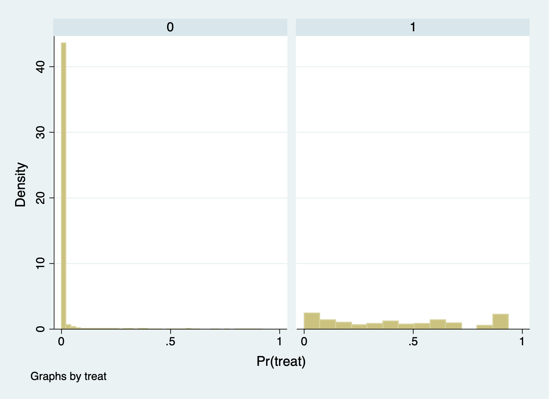 It seems that there is very little overlap for the common support assumption. It would be problematic to estimate the \(ATE\) and \(ATT\) without trimming to get common support.
1.2 Estimate the \(ATE\) and \(ATT\) without trimming
We will estimate the \(ATE\) and \(ATT\) with the teffects psmatch command. We will use the 5 nearest neighbors with the option nn(5). Note that Stata generates new variables defined by you. Here we are defining pstub_cps.
Estimate \(ATT\)
teffects psmatch (re78) (treat age agesq agecube educ edusq marr nodegree black ///
 hisp re74 re75 u74 u75 interaction1, logit), atet gen(pstub_cps) nn(5)
drop pstub_cps*
Treatment-effects estimation Number of obs = 16,177
Estimator : propensity-score matching Matches: requested = 5
Outcome model : matching min = 5
Treatment model: logit max = 26
------------------------------------------------------------------------------
| AI robust
re78 | Coefficient std. err. z P>|z| [95% conf. interval]
-------------+----------------------------------------------------------------
ATET |
treat |
(1 vs 0) | 1725.082 700.0583 2.46 0.014 352.9928 3097.171
------------------------------------------------------------------------------\(\widehat{ATT} = \$1,725.082\)
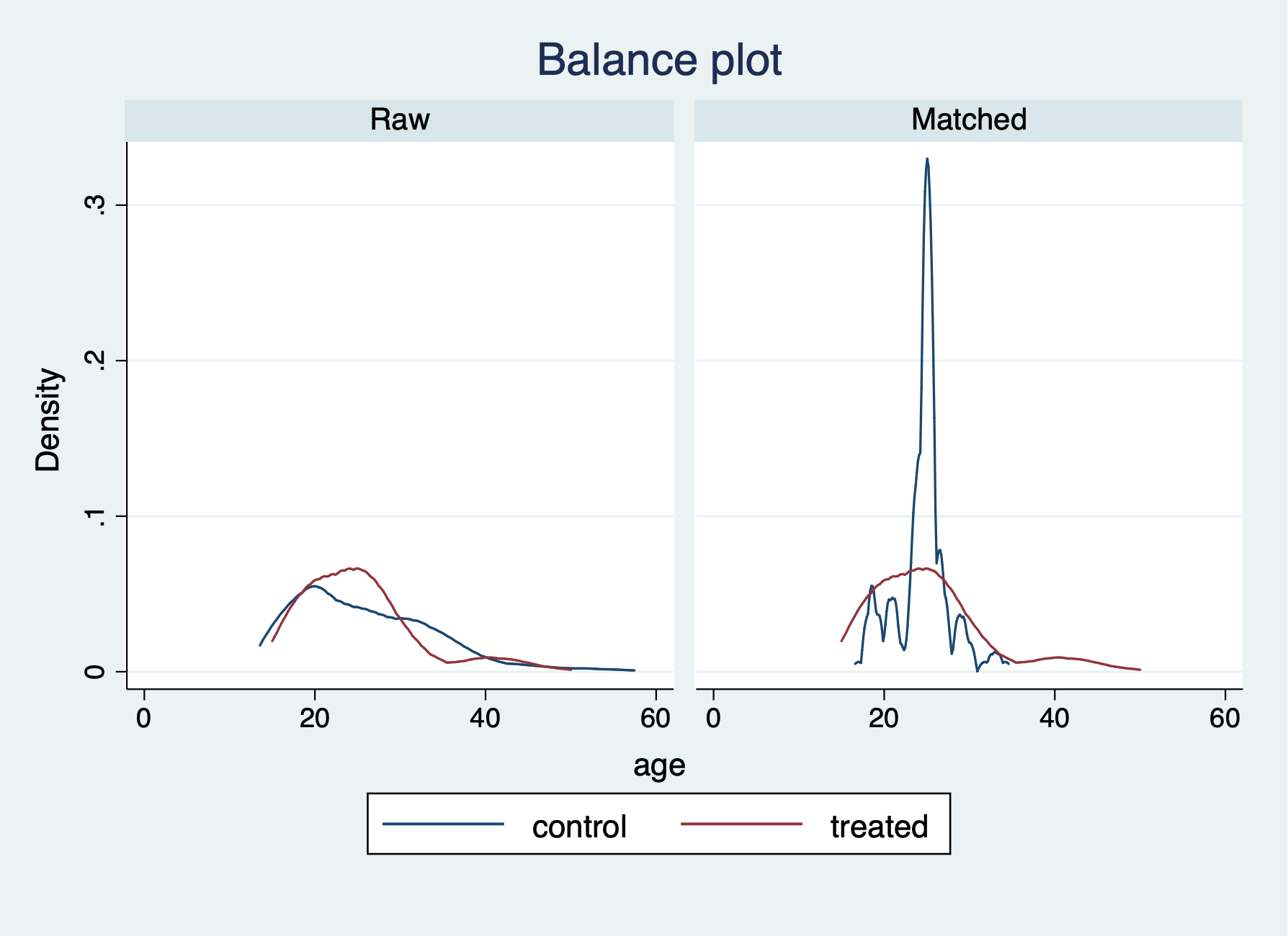
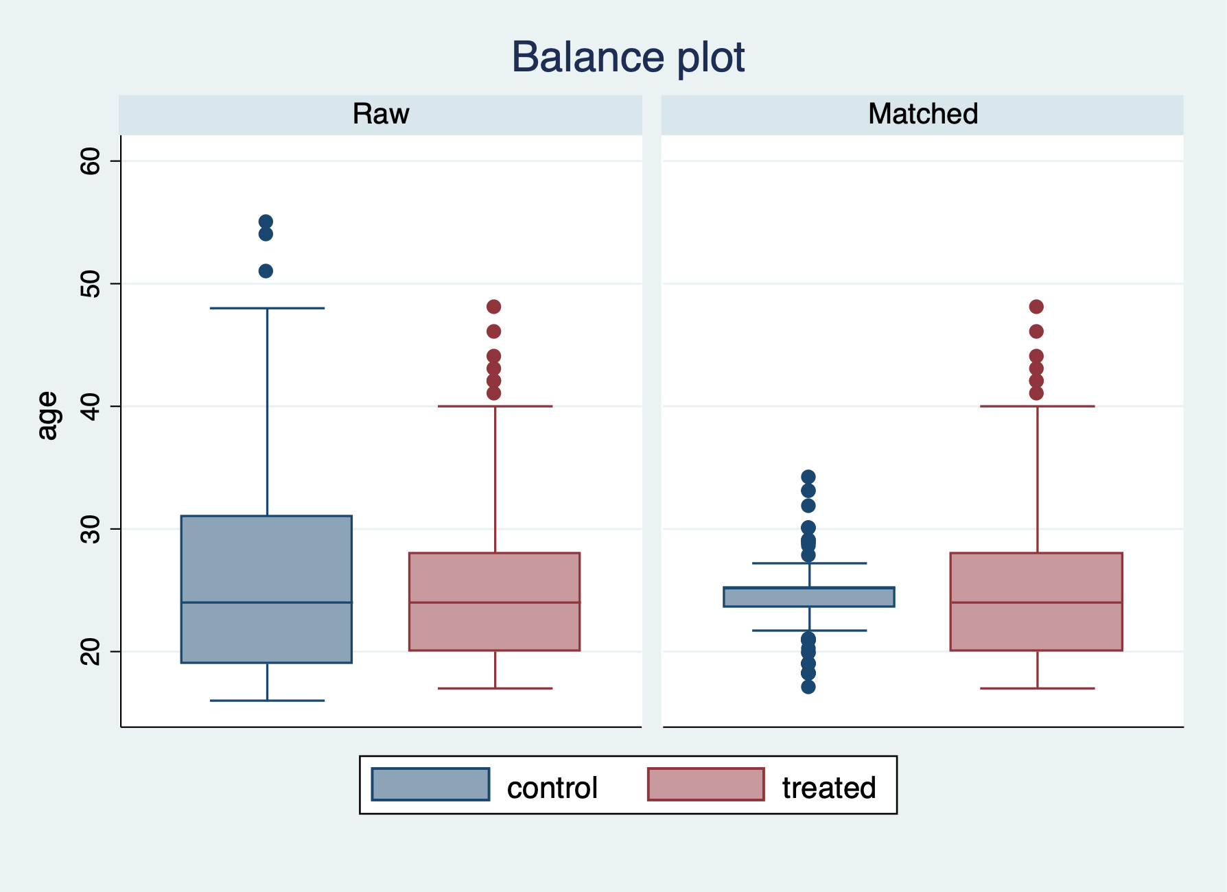
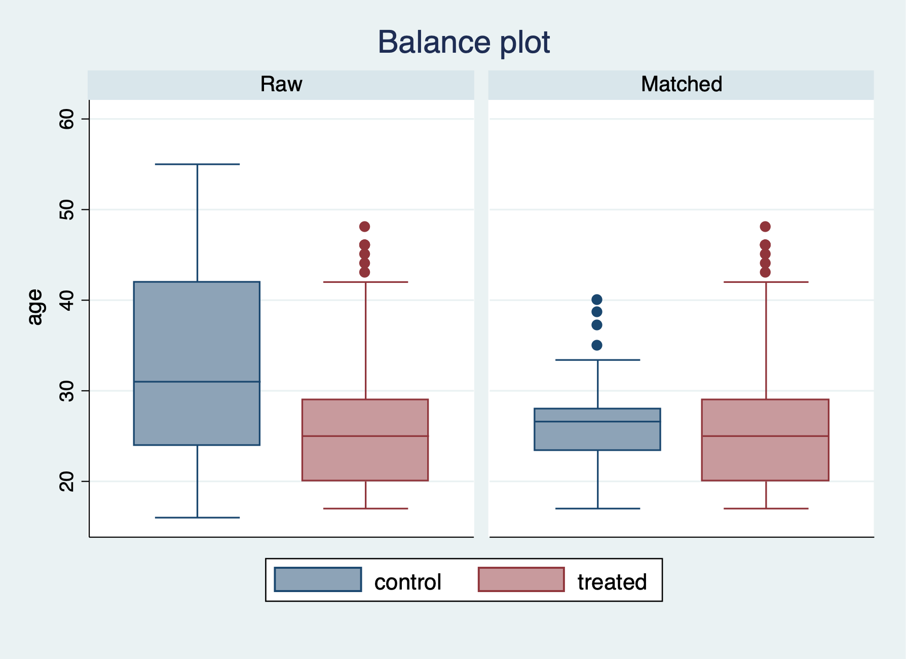
We have a few more options for checking the balance after the PSM with nearest neighbor of 5. We can use the teblance commands to check our balance. tebalance density will give us a distribution of propensity scores by our variable of choice between treatment and comparison. We can also use tebalance box that will give is a box-and-whisker chart for the propensity scores by our variable of choice between treatment and comparison.
Covariate balance summary

                         Raw      Matched
-----------------------------------------
Number of obs =       16,177          370
Treated obs   =          185          185
Control obs   =       15,992          185
-----------------------------------------

-----------------------------------------------------------------
                |           Means                  Variances
                |    Control     Treated       Control    Treated
----------------+------------------------------------------------
            age |   33.22524    25.81622      121.9968    51.1943
          agesq |   1225.906    717.3946      615814.1     185978
        agecube |   49305.85    21554.66      2.04e+09   4.40e+08
           educ |   12.02751    10.34595      8.241754   4.042714
          edusq |   152.9023    111.0595      4511.316   1544.795
           marr |   .7117309    .1891892      .2051829   .1542303
       nodegree |   .2958354    .7081081      .2083299   .2078143
          black |   .0735368    .8432432      .0681334   .1329025
           hisp |    .072036    .0594595       .066851    .056228
           re74 |    14016.8    2095.574      9.16e+07   2.39e+07
           re75 |    13650.8    1532.055      8.59e+07   1.04e+07
            u74 |   .1196223    .7081081      .1053194   .2078143
            u75 |   .1093047          .6      .0973632   .2413043
   interaction1 |   171147.6    22898.73      1.67e+10   3.29e+09
-----------------------------------------------------------------
After running tebalance summarize, we can see without trimming that our covariates are not really balanced between treatment and comparison groups.
Next, we will estimate the \(ATE\) with teffects psmatch.
teffects psmatch (re78) (treat age agesq agecube educ edusq marr nodegree black ///
 hisp re74 re75 u74 u75 interaction1, logit), ate gen(pstub_cps) nn(5)

drop pstub_cps*
We find that we have an error estimating the \(ATE\), since we lack common support.
1.3 Trim the data
We will use the trim the \(p\)-scores. All values below \(10\%\) and above \(90\%\) will be dropped.
We can see that the comparison group has a lot of observations with \(p\)-scores less than or equal to 0.1 (15,802), but we only drop 14 observations with \(p\)-scores greater than or equal 0.9.
(15,802 observations deleted)

(14 observations deleted)
1.4 Check for balance again
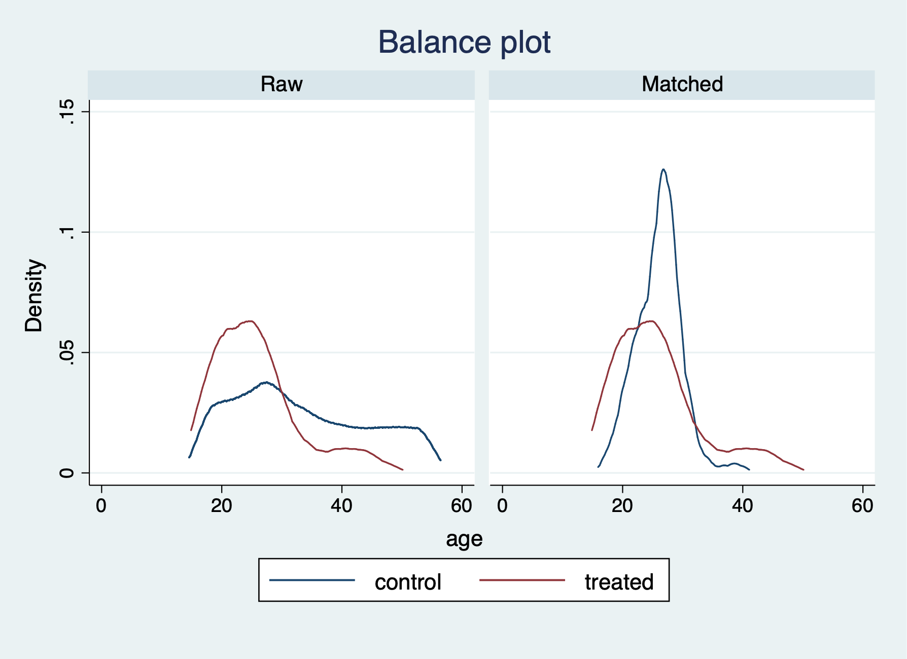
 We can now see we have better overlap between treatment and comparison after trimming the extreme values of the \(p\)-scores.
1.5 Reestimate the \(ATT\) and \(ATE\)
teffects psmatch (re78) (treat age agesq agecube educ edusq marr nodegree black ///
 hisp re74 re75 u74 u75 interaction1, logit), ate gen(pstub_cps) nn(5)

drop pstub_cps*
Treatment-effects estimation Number of obs = 361
Estimator : propensity-score matching Matches: requested = 5
Outcome model : matching min = 5
Treatment model: logit max = 8
------------------------------------------------------------------------------
| AI robust
re78 | Coefficient std. err. z P>|z| [95% conf. interval]
-------------+----------------------------------------------------------------
ATE |
treat |
(1 vs 0) | 1758.837 724.5845 2.43 0.015 338.6778 3178.997
------------------------------------------------------------------------------\(\widehat{ATE}= \$1758.84\)
teffects psmatch (re78) (treat age agesq agecube educ edusq marr nodegree black ///
 hisp re74 re75 u74 u75 interaction1, logit), atet gen(pstub_cps) nn(5)
Treatment-effects estimation Number of obs = 361
Estimator : propensity-score matching Matches: requested = 5
Outcome model : matching min = 5
Treatment model: logit max = 8
------------------------------------------------------------------------------
| AI robust
re78 | Coefficient std. err. z P>|z| [95% conf. interval]
-------------+----------------------------------------------------------------
ATET |
treat |
(1 vs 0) | 2519.446 866.7552 2.91 0.004 820.6375 4218.255
------------------------------------------------------------------------------\(\widehat{ATE}= \$2519.446\)
1.6 Recheck for balance
Covariate balance summary

                         Raw      Matched
-----------------------------------------
Number of obs =          361          266
Treated obs   =          133          133
Control obs   =          228          133
-----------------------------------------

-----------------------------------------------------------------
                |           Means                  Variances
                |    Control     Treated       Control    Treated
----------------+------------------------------------------------
            age |   25.93421     25.2406      64.98684   45.00228
          agesq |   737.2851    681.7519        237422   158499.2
        agecube |   22966.88    19825.29      6.03e+08   3.66e+08
           educ |   10.46491     10.2406      4.584667   3.850763
          edusq |   114.0789    108.6917      1830.681   1331.306
           marr |   .2192982    .1428571      .1719607   .1233766
       nodegree |   .6315789    .7518797       .233712   .1879699
          black |   .9342105    .9398496       .061732   .0569606
           hisp |   .0438596     .037594      .0421207   .0364548
           re74 |   2552.555    1560.604      1.93e+07   1.56e+07
           re75 |   1570.309    1002.193       7324536    3233917
            u74 |   .5570175    .7669173       .247836   .1801094
            u75 |   .4868421    .6390977      .2509274   .2323992
   interaction1 |   27361.94    16425.15      2.44e+09   1.81e+09
-----------------------------------------------------------------
Our balance is greatly improved after trimming the tail ends of the propensity scores.
Let’s check the variable age with tebalance density and tebalance box.