Chapter 2 Inverse Probability Weights

We will reload our treatment group and CPS comparison group, and use the teffects ipw command to estimate the $ATE$.

We will repull our data, estimate our $p$-score, and check our balance

*Get Data
use https://github.com/scunning1975/mixtape/raw/master/nsw_mixtape.dta, clear
drop if treat==0
append using https://github.com/scunning1975/mixtape/raw/master/cps_mixtape.dta

*Calculate Variables
gen agesq=age*age
gen agecube=age*age*age
gen edusq=educ*edu
gen u74 = 0 if re74!=.
replace u74 = 1 if re74==0
gen u75 = 0 if re75!=.
replace u75 = 1 if re75==0
gen interaction1 = educ*re74
gen re74sq=re74^2
gen re75sq=re75^2
gen interaction2 = u74*hisp

*Estimate the coefficients
logit treat age agesq agecube educ edusq marr nodegree black hisp re74 re75 u74 u75 interaction1 
predict pscore

* Checking mean propensity scores for treatment and control groups
sum pscore if treat==1, detail
sum pscore if treat==0, detail

* Now look at the propensity score distribution for treatment and control groups
histogram pscore, by(treat) binrescale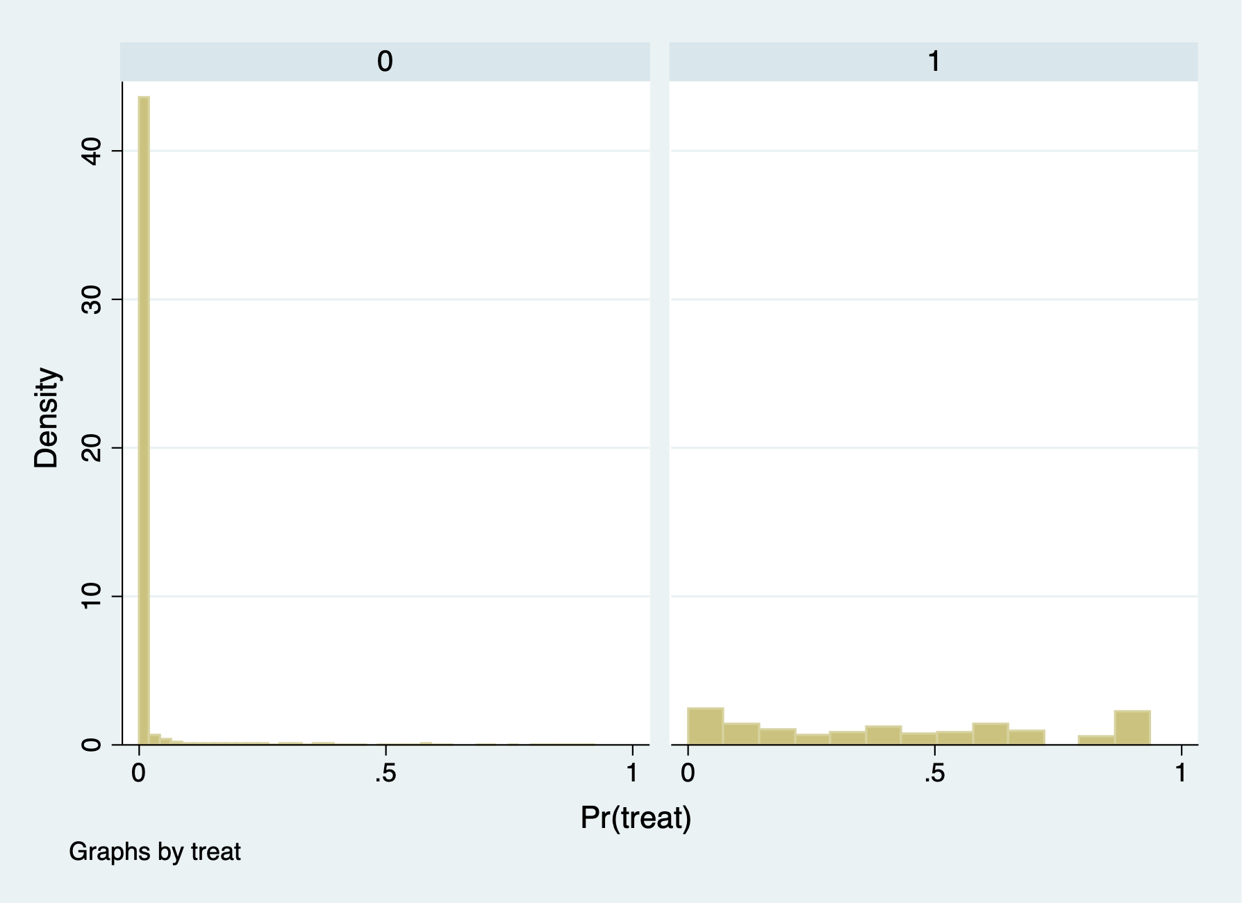

Histogram for IPW

2.1 Manual Calculate the $ATE$

We will manually calculate inverse probability weighting (IPW) with Propensity Scores. Please note that IPW is not matching, even though we use propensity scores.

IPW with Non-normalized Weights: \[ \widehat{ATE} = \frac{1}{n}*\sum_{n=1}^{N} \left( {\frac{Y_i*D_i}{\hat{p}(x)_i}} \right)-\frac{1}{n}*\sum_{n=1}^{N} \left( {\frac{Y_i*(1-D_i)}{1-\hat{p}(x)_i}} \right) \]

IPW with Normalized Weights:

\[ \widehat{ATE}=\left[\sum_{n=1}^{N}\frac{Y_i*D_i}{\hat{p}(x)_i} \right] / \left[\sum_{n=1}^{N}\frac{D_i}{\hat{p}(x)_i} \right] - \left[\sum_{n=1}^{N}\frac{Y_i*(1-D_i)}{(1-\hat{p}(x)_i)} \right] / \left[\sum_{n=1}^{N}\frac{(1-D_i)}{(1-\hat{p}(x)_i)} \right] \]

2.1.1 Calculate $E[Y^1]$ and $E[Y^0]$

First, we need to calculate normalization weights

gen d1=treat/pscore
gen d0=(1-treat)/(1-pscore)

Sum the inverse pscore

egen s1=sum(d1)
egen s0=sum(d0) 
gen total = _N
egen total_T = sum(treat)
egen total_C = sum(1-treat)

First, we will manually calculate $E[Y^1]$ with non-normalized weights using all the data. Calculate $E[Y^1]=\frac{1}{n}*\sum_{n=1}^{N}\frac{Y_i*D_i}{\hat{p}(x)_i}$

gen y1=treat*re78/pscore
egen y1_2 = sum(y1)
gen y1_3 = y1_2/total

Next, we will manually calculate $E[Y^0]$ with non-normalized weights using all the data. Calculate $E[Y^0]=\frac{1}{n}*\sum_{n=1}^{N}\frac{Y*(1-D_i)}{(1-\hat{p}(x)_i)}$

gen y0=(1-treat)*re78/(1-pscore) 
egen y0_2 = sum(y0)
gen y0_3 = y0_2/total

Then calculate the $ATE$ by taking the difference in $E[Y^1]-E[Y^0]$.

*Way 1
gen ht=y1-y0
*Way 2
gen ht2=y1_3-y0_3
*Same results
sum ht ht2

    Variable |        Obs        Mean    Std. dev.       Min        Max
-------------+---------------------------------------------------------
          ht |     16,177   -11876.79    127578.8  -99232.62   1.19e+07
         ht2 |     16,177   -11876.79           0  -11876.79  -11876.79

Now we will calculate the $ATE$ manually using normalized weights

*Way 1
replace y1=(treat*re78/pscore)/(s1/total)
replace y0=((1-treat)*re78/(1-pscore))/(s0/total)
*Way 2
replace y1_3=y1_2/s1
replace y0_3=y0_2/s0
*Get the estimated ATE
gen norm=y1-y0
gen norm2=y1_3-y0_3
*Same Results for ht:ht2 and norm:norm2
sum ht ht2 norm norm2

(140 real changes made)

(13,820 real changes made)

(16,177 real changes made)

(16,177 real changes made)

    Variable |        Obs        Mean    Std. dev.       Min        Max
-------------+---------------------------------------------------------
          ht |     16,177   -11876.79    127578.8  -99232.62   1.19e+07
         ht2 |     16,177   -11876.79           0  -11876.79  -11876.79
        norm |     16,177    -7238.14    332633.6  -99127.18   3.11e+07
       norm2 |     16,177    -7238.14           0   -7238.14   -7238.14

ATE under non-normalized weights is -$11,876. ATE under normalized weights is -$7,238.

Why are they so much different than the experimental research design estimates? Given that the mean $1-p(x)$ is close to 1, a lot of weight is given to $Y^0$. What we need to do is trim and recalculate.

2.1.2 Trim the data

We will drop our calculated variables and then trim our $p$-scores.

drop d1 d0 s1 s0 y1 y0 ht norm
drop if pscore <= 0.1 
drop if pscore >= 0.9

We will recalculate the non-normalized weights using trimmed data.

gen d1=treat/pscore
gen d0=(1-treat)/(1-pscore)
egen s1=sum(d1)
egen s0=sum(d0)

gen y1=treat*re78/pscore
gen y0=(1-treat)*re78/(1-pscore)
gen ht=y1-y0

We will recalculate the normalized weights using trimmed data.

replace y1=(treat*re78/pscore)/(s1/_N)
replace y0=((1-treat)*re78/(1-pscore))/(s0/_N)
gen norm=y1-y0
sum ht norm

(0 real changes made)

(0 real changes made)

(0 real changes made)

    Variable |        Obs        Mean    Std. dev.       Min        Max
-------------+---------------------------------------------------------
          ht |        361    2006.365    19656.33  -73545.45   131755.3
        norm |        361     1806.73    18967.72  -72480.23   126251.9

ATE under non-normalized weights is $2,006, while the estimated ATE under normalized weights is $1,807.

These are much closer to our experimental research design estimates.

2.2 Calculate $ATE$ and $ATT$ using teffects

Luckily, we have a built-in Stata command with teffects ipw, so we don’t need to manually calculate the $ATE$ everytime. (However, it is a good exercise to see how Stata calculate the estimate). The teffects command will also calculate our standard errors, as well.

We will reload our data, trim the data, and use the teffects ipw command. We will also trim our data, since we know that there is a lack of overlap at the tail ends of the estimated $p$-scores.

* Reload Data
use https://github.com/scunning1975/mixtape/raw/master/nsw_mixtape.dta, clear
drop if treat==0

*Now merge in the CPS controls from footnote 2 of Table 2 (Dehejia and Wahba 2002)
append using https://github.com/scunning1975/mixtape/raw/master/cps_mixtape.dta
gen agesq=age*age
gen agecube=age*age*age
gen edusq=educ*edu
gen u74 = 0 if re74!=.
replace u74 = 1 if re74==0
gen u75 = 0 if re75!=.
replace u75 = 1 if re75==0
gen interaction1 = educ*re74
gen re74sq=re74^2
gen re75sq=re75^2
gen interaction2 = u74*hisp

* Now estimate the propensity score
logit treat age agesq agecube educ edusq marr nodegree black hisp re74 re75 u74 u75 interaction1 
predict pscore

* Checking mean propensity scores for treatment and control groups
sum pscore if treat==1, detail
sum pscore if treat==0, detail

* Trimming the propensity score
drop if pscore <= 0.1 
drop if pscore >= 0.9

With the teffects command, we need to specify ipw for inverse probability weights and we need to use the option logit to tell Stata to calculate the $p$-scores using a logistic regresion. In addition, we will use the option osample to look for any overlap between treatment and comparison. Finally, we will use the option atet to specify that we want to estimate the $ATT$.

teffects ipw (re78) (treat age agesq agecube educ edusq marr nodegree ///
black hisp re74 re75 u74 u75 interaction1, logit), osample(overlap) atet
capture drop overlap

Iteration 0:  EE criterion = 1.354e-21  
Iteration 1:  EE criterion = 7.719e-24  

Treatment-effects estimation                    Number of obs     =        361
Estimator      : inverse-probability weights
Outcome model  : weighted mean
Treatment model: logit
------------------------------------------------------------------------------
             |               Robust
        re78 | Coefficient  std. err.      z    P>|z|     [95% conf. interval]
-------------+----------------------------------------------------------------
ATET         |
       treat |
   (1 vs 0)  |   2646.866     892.23     2.97   0.003     898.1271    4395.604
-------------+----------------------------------------------------------------
POmean       |
       treat |
          0  |   3791.931   514.4672     7.37   0.000     2783.593    4800.268
------------------------------------------------------------------------------

The ATT is estimated at $2,647

Before we calculate the $ATE$, we need to rescale the dependent variable for concavity of logit. We will do so by dividing re78 by 1000 dollars

The ATE is estimated at $1,611

gen re78_scaled = re78/1000
teffects ipw (re78_scaled) (treat age agesq agecube educ edusq marr nodegree ///
black hisp re74 re75 u74 u75 interaction1, logit), osample(overlap) ate

Iteration 0:  EE criterion = 1.348e-21  
Iteration 1:  EE criterion = 2.117e-30  

Treatment-effects estimation                    Number of obs     =        361
Estimator      : inverse-probability weights
Outcome model  : weighted mean
Treatment model: logit
------------------------------------------------------------------------------
             |               Robust
 re78_scaled | Coefficient  std. err.      z    P>|z|     [95% conf. interval]
-------------+----------------------------------------------------------------
ATE          |
       treat |
   (1 vs 0)  |   1.610583    .673642     2.39   0.017     .2902694    2.930898
-------------+----------------------------------------------------------------
POmean       |
       treat |
          0  |   4.222608    .376673    11.21   0.000     3.484342    4.960874
------------------------------------------------------------------------------

Matching Methods

Chapter 2 Inverse Probability Weights

2.1 Manual Calculate the \(ATE\)

2.1.1 Calculate \(E[Y^1]\) and \(E[Y^0]\)

2.1.2 Trim the data

2.2 Calculate \(ATE\) and \(ATT\) using teffects