Chapter 2 Fixed Effects (Within) Estimator
We will implement the fixed effects (within) estimator. We will need to use the xtset command to establish our unit of analysis dimension and our time dimension in our panel data. Our main stata command to implement a FD is xtreg with the option fe. It is important to include the option fe. If you forget, your model will be a random effects model.
2.1 Union Premium
Lesson: we can control for ability and preference for unionization to control for unobserved time-invariant confounders.
We want to estimate the union premium, and we will use a fixed effects (within) estimator to control for time-invariant heterogeneity, such as ability and performance.
\[ ln(wage_{i,t}) = \beta_0 + \beta_1 edu_{i,t} + \beta_2 exp_{i,t} + \beta_3 exp^2_{i,t} + \beta_4 Black_{i} + \beta_7 South_{i,t} \\ + \beta_8 married_{i,t} + union_{i,t} + a_t + a_i + \varepsilon_{i,t} \]
Set the Panel and estimate the Pooled OLS model
       panel variable:  nr (strongly balanced)
        time variable:  year, 1980 to 1987
                delta:  1 unit

      Source |       SS           df       MS      Number of obs   =     4,360
-------------+----------------------------------   F(14, 4345)     =     73.43
       Model |  236.577196        14  16.8983712   Prob > F        =    0.0000
    Residual |  999.952446     4,345  .230138653   R-squared       =    0.1913
-------------+----------------------------------   Adj R-squared   =    0.1887
       Total |  1236.52964     4,359  .283672779   Root MSE        =    .47973

------------------------------------------------------------------------------
       lwage |      Coef.   Std. Err.      t    P>|t|     [95% Conf. Interval]
-------------+----------------------------------------------------------------
        educ |   .0895815   .0051762    17.31   0.000     .0794334    .0997295
       exper |   .0665418   .0136722     4.87   0.000     .0397372    .0933463
     expersq |  -.0023832   .0008183    -2.91   0.004    -.0039875   -.0007789
     1.black |  -.1275978   .0236068    -5.41   0.000    -.1738791   -.0813165
     1.south |  -.0529354   .0155534    -3.40   0.001    -.0834281   -.0224428
   1.married |   .1122106   .0157149     7.14   0.000     .0814014    .1430198
     1.union |   .1802554   .0171339    10.52   0.000     .1466642    .2138466
       1.d81 |    .058693   .0303147     1.94   0.053    -.0007393    .1181253
       1.d82 |   .0638086   .0331714     1.92   0.054    -.0012242    .1288414
       1.d83 |   .0633355   .0366129     1.73   0.084    -.0084444    .1351153
       1.d84 |   .0915252   .0400387     2.29   0.022     .0130289    .1700216
       1.d85 |   .1105424   .0432973     2.55   0.011     .0256575    .1954272
       1.d86 |   .1437822   .0463663     3.10   0.002     .0528806    .2346837
       1.d87 |   .1756699   .0493736     3.56   0.000     .0788725    .2724673
       _cons |   .1333638   .0774193     1.72   0.085    -.0184175     .285145
------------------------------------------------------------------------------
If we use FE or FD, we cannot assess race, education, or experience since they remain constant.
FE Within.
note: educ omitted because of collinearity
note: 1.black omitted because of collinearity
note: 1.d87 omitted because of collinearity

Fixed-effects (within) regression               Number of obs     =      4,360
Group variable: nr                              Number of groups  =        545

R-sq:                                           Obs per group:
     within  = 0.1815                                         min =          8
     between = 0.0009                                         avg =        8.0
     overall = 0.0497                                         max =          8

                                                F(11,3804)        =      76.71
corr(u_i, Xb)  = -0.1739                        Prob > F          =     0.0000

------------------------------------------------------------------------------
       lwage |      Coef.   Std. Err.      t    P>|t|     [95% Conf. Interval]
-------------+----------------------------------------------------------------
        educ |          0  (omitted)
       exper |   .1313318   .0098277    13.36   0.000     .1120638    .1505999
     expersq |  -.0051475   .0007043    -7.31   0.000    -.0065284   -.0037666
     1.black |          0  (omitted)
     1.south |   .1018493   .0479605     2.12   0.034     .0078186      .19588
   1.married |   .0462057   .0183034     2.52   0.012     .0103203     .082091
     1.union |   .0809394   .0193065     4.19   0.000     .0430874    .1187914
       1.d81 |   .0190821   .0203532     0.94   0.349    -.0208222    .0589864
       1.d82 |  -.0117214   .0202191    -0.58   0.562    -.0513627    .0279199
       1.d83 |  -.0425071   .0203126    -2.09   0.036    -.0823318   -.0026825
       1.d84 |  -.0378955   .0203069    -1.87   0.062    -.0777089    .0019179
       1.d85 |  -.0427598   .0202377    -2.11   0.035    -.0824377   -.0030819
       1.d86 |  -.0276303   .0203773    -1.36   0.175    -.0675818    .0123211
       1.d87 |          0  (omitted)
       _cons |   .9952994    .033587    29.63   0.000      .929449     1.06115
-------------+----------------------------------------------------------------
     sigma_u |  .40924292
     sigma_e |  .35082825
         rho |  .57640294   (fraction of variance due to u_i)
------------------------------------------------------------------------------
F test that all u_i=0: F(544, 3804) = 9.54                   Prob > F = 0.0000
Compare with esttab
                      (1)             (2)
                      OLS          Within
--------------------------------------------
educ               0.0896***            0
                (0.00518)             (.)

exper              0.0665***        0.131***
                 (0.0137)       (0.00983)

expersq          -0.00238**      -0.00515***
               (0.000818)      (0.000704)

0.black                 0               0
                      (.)             (.)

1.black            -0.128***            0
                 (0.0236)             (.)

0.south                 0               0
                      (.)             (.)

1.south           -0.0529***        0.102*
                 (0.0156)        (0.0480)

1.married           0.112***       0.0462*
                 (0.0157)        (0.0183)

1.union             0.180***       0.0809***
                 (0.0171)        (0.0193)

1.d81              0.0587          0.0191
                 (0.0303)        (0.0204)

1.d82              0.0638         -0.0117
                 (0.0332)        (0.0202)

1.d83              0.0633         -0.0425*
                 (0.0366)        (0.0203)

1.d84              0.0915*        -0.0379
                 (0.0400)        (0.0203)

1.d85               0.111*        -0.0428*
                 (0.0433)        (0.0202)

1.d86               0.144**       -0.0276
                 (0.0464)        (0.0204)

1.d87               0.176***            0
                 (0.0494)             (.)

_cons               0.133           0.995***
                 (0.0774)        (0.0336)
--------------------------------------------
N                    4360            4360
F                   73.43           76.71
r2                  0.191           0.182
--------------------------------------------
Standard errors in parentheses
* p<0.05, ** p<0.01, *** p<0.001
After controlling for time-invariant individual fixed effects the Pooled OLS is seen to be upward biased. The union wage premium is about 19.7% with the Pooled OLS model, while the union wage premium is estimated to be 8.4% after accounting for individual fixed effects.
Pooled OLS Wage Premium Estimate
19.752317FE Within Wage Premium Estimate
8.4305206Plot the Coefficients of Interest Credit: John Kane: Making Regression Coefficients Plots in Stata
quietly reg lwage c.edu exper expersq i.black i.south i.married i.union i.d8*
estimates store pooled
quietly xtreg lwage c.edu i.black i.south i.married i.union i.d8*, fe
estimates store fe
coefplot (pooled, label("{bf:Pooled OLS}") mcolor(midblue) mlcolor(cyan) ///
      ciopts(lcolor(magenta midblue))) /// options for first group
      (fe, label("{bf: Within}") mcolor(green) mlcolor(lime) ///
      ciopts(lcolor(lime green))), /// options for second group
      title(Union and Marriage Wage Premiums) ///
      drop(_cons 1.d* 0.black 0.south) ///
      xline(0, lcolor(red) lwidth(medium)) scheme(jet_white) ///
      xtitle("{bf: Effect of Union}") ///
      graphregion(margin(small)) ///
      coeflabels(educ="Education" exper="Experience" expersq="Experience Squared" ///
      1.black="Black" 1.south="South" 1.married="Married" ///
      1.union="Union") ///
      msize(large) mcolor(%85) mlwidth(medium) msymbol(circle) /// marker options
      levels(95 90) ciopts(lwidth(medthick thick) recast(rspike rcap)) ///ci options for all groups
      legend(ring(1) col(1) pos(3) size(medsmall))
      graph export "/Users/Sam/Desktop/Econ 645/Stata/week4_union_wage_premium.png", replace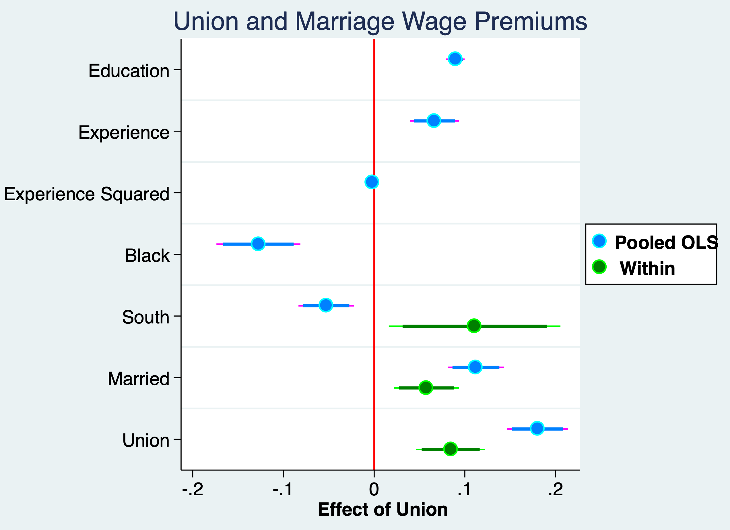
2.2 Has returns to education changed over time
Lesson: We can interact time binaries with continuous time-invariant data to see if returns to education have changed over time<
With fixed effects or first differencing, we cannot assess time-invariant variables. Variables that do not vary over time, such as sex, race, or education (assuming) education is static. But, if we interact education with time binaries, we can assess whether returns to education have increased over time.
We can test to see if returns to education are constant over time.
Vella and Verbeek (1998) estimate to see if the returns to education have change over time. We have some variables that are not time-invariant, such as union status and marital status. Experience does growth but it grows at a constant rate. We have a few variable that do not (or we would expect not to change), such as race and education (for older workers).
We use the natural log of wages, which has nice properties, such as being are more normally distributed and providing elasticities. It also can take care of inflation when we add time period binaries.
Set up the Panel
Pooled OLS
      Source |       SS           df       MS      Number of obs   =     4,360
-------------+----------------------------------   F(19, 4340)     =     50.92
       Model |  225.412805        19  11.8638318   Prob > F        =    0.0000
    Residual |  1011.11684     4,340   .23297623   R-squared       =    0.1823
-------------+----------------------------------   Adj R-squared   =    0.1787
       Total |  1236.52964     4,359  .283672779   Root MSE        =    .48268

------------------------------------------------------------------------------
       lwage |      Coef.   Std. Err.      t    P>|t|     [95% Conf. Interval]
-------------+----------------------------------------------------------------
        educ |    .081673   .0125675     6.50   0.000     .0570343    .1063117
       1.d81 |  -.0356958    .199359    -0.18   0.858    -.4265413    .3551497
       1.d82 |  -.0315288   .1998095    -0.16   0.875    -.4232575       .3602
       1.d83 |  -.0342801   .2007839    -0.17   0.864    -.4279192    .3593589
       1.d84 |   .0242933   .2025167     0.12   0.905    -.3727429    .4213294
       1.d85 |   .0058838   .2052301     0.03   0.977    -.3964719    .4082395
       1.d86 |   .0251586   .2092184     0.12   0.904    -.3850164    .4353336
       1.d87 |   .0372565   .2148364     0.17   0.862    -.3839326    .4584456
             |
  d81#c.educ |
          1  |   .0084448   .0167792     0.50   0.615     -.024451    .0413407
             |
  d82#c.educ |
          1  |   .0088899   .0168742     0.53   0.598    -.0241921     .041972
             |
  d83#c.educ |
          1  |   .0093544   .0170326     0.55   0.583    -.0240381     .042747
             |
  d84#c.educ |
          1  |   .0070671   .0172551     0.41   0.682    -.0267617    .0408958
             |
  d85#c.educ |
          1  |   .0104027   .0175306     0.59   0.553    -.0239662    .0447716
             |
  d86#c.educ |
          1  |   .0116562   .0178614     0.65   0.514    -.0233613    .0466737
             |
  d87#c.educ |
          1  |   .0134166   .0182525     0.74   0.462    -.0223676    .0492008
             |
       exper |   .0568876   .0154436     3.68   0.000     .0266102     .087165
     expersq |   -.001919   .0009455    -2.03   0.042    -.0037726   -.0000654
   1.married |   .1229473   .0155752     7.89   0.000     .0924119    .1534827
     1.union |   .1720565   .0171378    10.04   0.000     .1384575    .2056554
       _cons |   .2175863   .1641736     1.33   0.185    -.1042777    .5394503
------------------------------------------------------------------------------
Fixed Effects (Within)
note: educ omitted because of collinearity

Fixed-effects (within) regression               Number of obs     =      4,360
Group variable: nr                              Number of groups  =        545

R-sq:                                           Obs per group:
     within  = 0.1708                                         min =          8
     between = 0.1900                                         avg =        8.0
     overall = 0.1325                                         max =          8

                                                F(16,3799)        =      48.91
corr(u_i, Xb)  = 0.0991                         Prob > F          =     0.0000

------------------------------------------------------------------------------
       lwage |      Coef.   Std. Err.      t    P>|t|     [95% Conf. Interval]
-------------+----------------------------------------------------------------
        educ |          0  (omitted)
       1.d81 |  -.0224158   .1458885    -0.15   0.878    -.3084431    .2636114
       1.d82 |  -.0057611   .1458558    -0.04   0.968    -.2917243    .2802021
       1.d83 |   .0104297   .1458579     0.07   0.943    -.2755377    .2963971
       1.d84 |   .0843743   .1458518     0.58   0.563    -.2015811    .3703297
       1.d85 |   .0497253   .1458602     0.34   0.733    -.2362465    .3356971
       1.d86 |   .0656064   .1458917     0.45   0.653    -.2204273    .3516401
       1.d87 |   .0904448   .1458505     0.62   0.535     -.195508    .3763977
             |
  d81#c.educ |
          1  |   .0115854   .0122625     0.94   0.345    -.0124562    .0356271
             |
  d82#c.educ |
          1  |   .0147905   .0122635     1.21   0.228    -.0092533    .0388342
             |
  d83#c.educ |
          1  |   .0171182   .0122633     1.40   0.163    -.0069251    .0411615
             |
  d84#c.educ |
          1  |   .0165839   .0122657     1.35   0.176     -.007464    .0406319
             |
  d85#c.educ |
          1  |   .0237085   .0122738     1.93   0.053    -.0003554    .0477725
             |
  d86#c.educ |
          1  |   .0274123    .012274     2.23   0.026     .0033481    .0514765
             |
  d87#c.educ |
          1  |   .0304332   .0122723     2.48   0.013     .0063722    .0544942
             |
   1.married |   .0548205   .0184126     2.98   0.003      .018721      .09092
     1.union |   .0829785   .0194461     4.27   0.000     .0448527    .1211042
       _cons |   1.362459   .0162385    83.90   0.000     1.330622    1.394296
-------------+----------------------------------------------------------------
     sigma_u |  .37264193
     sigma_e |  .35335713
         rho |  .52654439   (fraction of variance due to u_i)
------------------------------------------------------------------------------
F test that all u_i=0: F(544, 3799) = 8.09                   Prob > F = 0.0000
If we use FE or FD, we cannot assess race, education, or experience since they remain constant, but we can include dummy interactions.
These are changes in the returns to education compared to the base year of 1980 And only \(1987 * education\) and \(1986 * education\) appear to be insignificant
Compare
                      (1)             (2)
                      OLS          Within
--------------------------------------------
educ               0.0817***            0
                 (0.0126)             (.)

1.d81             -0.0357         -0.0224
                  (0.199)         (0.146)

1.d82             -0.0315        -0.00576
                  (0.200)         (0.146)

1.d83             -0.0343          0.0104
                  (0.201)         (0.146)

1.d84              0.0243          0.0844
                  (0.203)         (0.146)

1.d85             0.00588          0.0497
                  (0.205)         (0.146)

1.d86              0.0252          0.0656
                  (0.209)         (0.146)

1.d87              0.0373          0.0904
                  (0.215)         (0.146)

1.d81#c.educ      0.00844          0.0116
                 (0.0168)        (0.0123)

1.d82#c.educ      0.00889          0.0148
                 (0.0169)        (0.0123)

1.d83#c.educ      0.00935          0.0171
                 (0.0170)        (0.0123)

1.d84#c.educ      0.00707          0.0166
                 (0.0173)        (0.0123)

1.d85#c.educ       0.0104          0.0237
                 (0.0175)        (0.0123)

1.d86#c.educ       0.0117          0.0274*
                 (0.0179)        (0.0123)

1.d87#c.educ       0.0134          0.0304*
                 (0.0183)        (0.0123)

exper              0.0569***
                 (0.0154)

expersq          -0.00192*
               (0.000945)

1.married           0.123***       0.0548**
                 (0.0156)        (0.0184)

1.union             0.172***       0.0830***
                 (0.0171)        (0.0194)

_cons               0.218           1.362***
                  (0.164)        (0.0162)
--------------------------------------------
N                    4360            4360
F                   50.92           48.91
r2                  0.182           0.171
--------------------------------------------
Standard errors in parentheses
* p<0.05, ** p<0.01, *** p<0.001
Returns to education have increased by about 3.1% between 1987 and 1980.
3.0866798Plot the Coefficients
quietly reg lwage c.edu##i.d8* exper expersq i.married i.union
estimates store pooled
quietly xtreg lwage c.edu##i.d8* i.married i.union, fe
estimates store fe
coefplot ///
      (pooled, label("{bf:Pooled OLS}") mcolor(midblue) mlcolor(cyan) ///
        ciopts(lcolor(magenta midblue))) /// options for first group
      (fe, label("{bf: Within}") mcolor(green) mlcolor(lime) ///
        ciopts(lcolor(lime green))), /// options for second gropu
      title("Change in Return to Education") ///
      keep(educ 1.d81#c.educ 1.d82#c.educ 1.d83#c.educ 1.d84#c.educ ///
        1.d85#c.educ 1.d86#c.educ 1.d87#c.educ) ///
      xline(0, lcolor(red) lwidth(medium)) scheme(jet_white) ///
      xtitle("{bf: Coefficients}") ///
      graphregion(margin(small)) ///
      coeflabels(educ="Education" 1.d81#c.educ="1981 Returns" ///
        1.d82#c.educ="1982 Returns" 1.d83#c.educ="1983 Returns" ///
        1.d84#c.educ="1984 Returns" 1.d85#c.educ="1985 Returns" ///
        1.d86#c.educ="1986 Returns" 1.d87#c.educ="1987 Returns") ///
      msize(large) mcolor(%85) mlwidth(medium) msymbol(circle) /// marker options
      levels(95 90) ciopts(lwidth(medthick thick) recast(rspike rcap)) ///ci options for all groups
      legend(ring(1) col(1) pos(3) size(medsmall))
    graph export "/Users/Sam/Desktop/Econ 645/Stata/week4_edu_returns.png", replace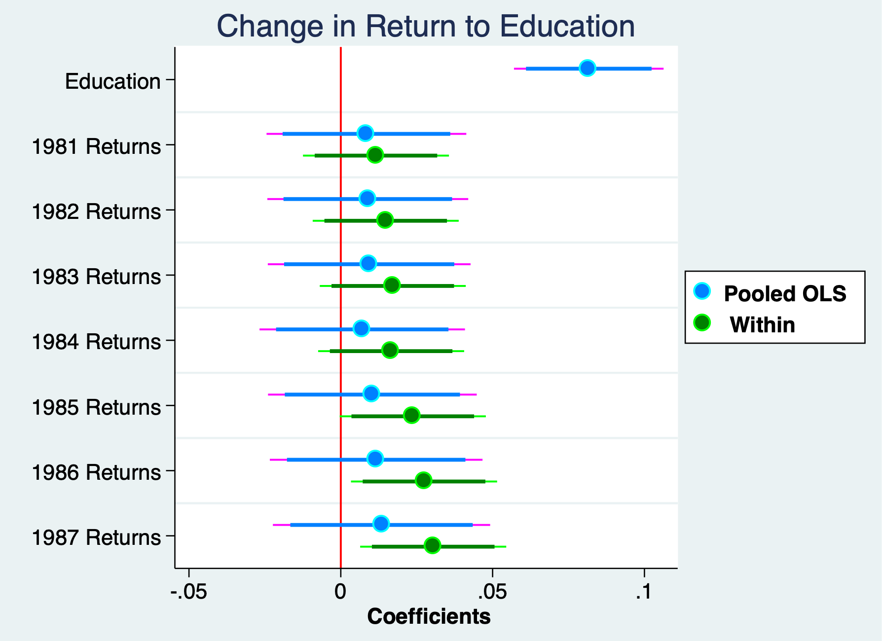
Test for Serial Correlation
Test for Serial Correlation. Use the option residuals or resid to get post-estimation residuals. If you don’t specify resid, Stata will return ( hat_{y} ) instead of ( hat_{u} )
Our null hypothesis is that there is no serial correlation or the coefficient on our lagged residuals is zero. We’ll regress u on lag of u AR(1) model without a constant
      Source |       SS           df       MS      Number of obs   =     3,815
-------------+----------------------------------   F(1, 3814)      =   2181.06
       Model |  332.737937         1  332.737937   Prob > F        =    0.0000
    Residual |  581.856111     3,814  .152557973   R-squared       =    0.3638
-------------+----------------------------------   Adj R-squared   =    0.3636
       Total |  914.594048     3,815  .239736317   Root MSE        =    .39059

------------------------------------------------------------------------------
           u |      Coef.   Std. Err.      t    P>|t|     [95% Conf. Interval]
-------------+----------------------------------------------------------------
           u |
         L1. |   .5857228   .0125418    46.70   0.000     .5611336     .610312
------------------------------------------------------------------------------
We can see that we have positive serial correlation since the coefficient on our lagged residual is positive and statistically significant. We will need to cluster our standard errors to account for the positive serial correlation.
Dealing with Heteroskedasticity and Serial Correlation
For heteroskedasticity, we will need to use heteroskedasticity-robust standard errors by using the robust option.
For serial correlation, we will need to cluster our standard errors. We will cluster the standard errors at the unit of analysis level.
eststo nocluster: quietly xtreg lwage c.edu##i.d8* i.married i.union, fe
eststo clustered: quietly xtreg lwage c.edu##i.d8* i.married i.union, fe robust cluster(nr)

esttab nocluster clustered, mtitle ("FE" "FE Clustered") drop(0.*) se
(1) (2)
FE FE Clustered
--------------------------------------------
educ 0 0
(.) (.)
1.d81 -0.0224 -0.0224
(0.146) (0.144)
1.d82 -0.00576 -0.00576
(0.146) (0.139)
1.d83 0.0104 0.0104
(0.146) (0.154)
1.d84 0.0844 0.0844
(0.146) (0.159)
1.d85 0.0497 0.0497
(0.146) (0.157)
1.d86 0.0656 0.0656
(0.146) (0.171)
1.d87 0.0904 0.0904
(0.146) (0.157)
1.d81#c.educ 0.0116 0.0116
(0.0123) (0.0122)
1.d82#c.educ 0.0148 0.0148
(0.0123) (0.0118)
1.d83#c.educ 0.0171 0.0171
(0.0123) (0.0131)
1.d84#c.educ 0.0166 0.0166
(0.0123) (0.0138)
1.d85#c.educ 0.0237 0.0237
(0.0123) (0.0136)
1.d86#c.educ 0.0274* 0.0274
(0.0123) (0.0147)
1.d87#c.educ 0.0304* 0.0304*
(0.0123) (0.0135)
1.married 0.0548** 0.0548*
(0.0184) (0.0212)
1.union 0.0830*** 0.0830***
(0.0194) (0.0230)
_cons 1.362*** 1.362***
(0.0162) (0.0203)
--------------------------------------------
N 4360 4360
--------------------------------------------
Standard errors in parentheses
* p<0.05, ** p<0.01, *** p<0.0012.3 Rental Prices
Exercise 1: Compare Pooled OLS, First Difference, and Fixed Effects Within
Get the data here: rental.dta
The data on rental prices and other variables in college towns from 1980 to 1990. Do more students affect the prices? The general model with unobserved fixed effects is \[ ln(rent_{i,t}) = \beta_0 + \delta_0 y90_t + \beta_1 ln(pop_{i,t})+\beta_2 ln(avginc_{i,t})+\beta_4 pctstu_{i,t} + a_t + a_i + \varepsilon_{i,t} \] Where pop is city population, avginc is average income, pctstu is the student percent of the population, and rent is the nominal rental prices
- Estimate a Pooled OLS. What does the estimate on y90 tell you?
- Are there concerns with the standard errors in the Pooled OLS?
- Use a First difference model. Does the coefficient on b3 change?
- Use a FE Within model. Are the results the same as the FD model?
Set the Panel
       panel variable:  city (strongly balanced)
        time variable:  year, 80 to 90
                delta:  10 units
Pooled OLS
Linear regression                               Number of obs     =        128
                                                F(4, 123)         =     223.26
                                                Prob > F          =     0.0000
                                                R-squared         =     0.8613
                                                Root MSE          =     .12592

------------------------------------------------------------------------------
             |               Robust
       lrent |      Coef.   Std. Err.      t    P>|t|     [95% Conf. Interval]
-------------+----------------------------------------------------------------
       1.y90 |   .2622267   .0579584     4.52   0.000     .1475017    .3769517
        lpop |   .0406863   .0223732     1.82   0.071       -.0036    .0849726
     lavginc |   .5714461   .0989016     5.78   0.000     .3756765    .7672157
      pctstu |   .0050436   .0011488     4.39   0.000     .0027696    .0073176
       _cons |  -.5688069   .8506229    -0.67   0.505    -2.252563    1.114949
------------------------------------------------------------------------------
First Difference
note: 1.y90 omitted because of collinearity

      Source |       SS           df       MS      Number of obs   =        64
-------------+----------------------------------   F(3, 60)        =      9.51
       Model |  .231738668         3  .077246223   Prob > F        =    0.0000
    Residual |  .487362198        60  .008122703   R-squared       =    0.3223
-------------+----------------------------------   Adj R-squared   =    0.2884
       Total |  .719100867        63  .011414299   Root MSE        =    .09013

------------------------------------------------------------------------------
     D.lrent |      Coef.   Std. Err.      t    P>|t|     [95% Conf. Interval]
-------------+----------------------------------------------------------------
       1.y90 |          0  (omitted)
             |
        lpop |
         D1. |   .0722456   .0883426     0.82   0.417     -.104466    .2489571
             |
     lavginc |
         D1. |   .3099605   .0664771     4.66   0.000     .1769865    .4429346
             |
      pctstu |
         D1. |   .0112033   .0041319     2.71   0.009     .0029382    .0194684
             |
       _cons |   .3855214   .0368245    10.47   0.000     .3118615    .4591813
------------------------------------------------------------------------------
Fixed Effects
Fixed-effects (within) regression               Number of obs     =        128
Group variable: city                            Number of groups  =         64

R-sq:                                           Obs per group:
     within  = 0.9765                                         min =          2
     between = 0.2173                                         avg =        2.0
     overall = 0.7597                                         max =          2

                                                F(4,60)           =     624.15
corr(u_i, Xb)  = -0.1297                        Prob > F          =     0.0000

------------------------------------------------------------------------------
       lrent |      Coef.   Std. Err.      t    P>|t|     [95% Conf. Interval]
-------------+----------------------------------------------------------------
       1.y90 |   .3855214   .0368245    10.47   0.000     .3118615    .4591813
        lpop |   .0722456   .0883426     0.82   0.417     -.104466    .2489571
     lavginc |   .3099605   .0664771     4.66   0.000     .1769865    .4429346
      pctstu |   .0112033   .0041319     2.71   0.009     .0029382    .0194684
       _cons |   1.409384   1.167238     1.21   0.232    -.9254394    3.744208
-------------+----------------------------------------------------------------
     sigma_u |  .15905877
     sigma_e |  .06372873
         rho |   .8616755   (fraction of variance due to u_i)
------------------------------------------------------------------------------
F test that all u_i=0: F(63, 60) = 6.67                      Prob > F = 0.0000