Chapter 1 Unit Roots
Lesson: when we have a unit root process or Time Series integrated of order one \(I(1)\) we can use a first difference to transform the time series into a weakly dependent and often stationary process.
1.1 Example: Revisit Fertility
Set the time series
/Users/Sam/Desktop/Econ 645/Data/Wooldridge

        time variable:  year, 1913 to 1984
                delta:  1 unit
Plot the Graph
twoway line gfr year, title("General Fertility Rate") ytitle("Children Born per 1,000 CBA Women") xtitle("Year")
graph export "/Users/Sam/Desktop/Econ 645/Stata/week_11_i1.png", replace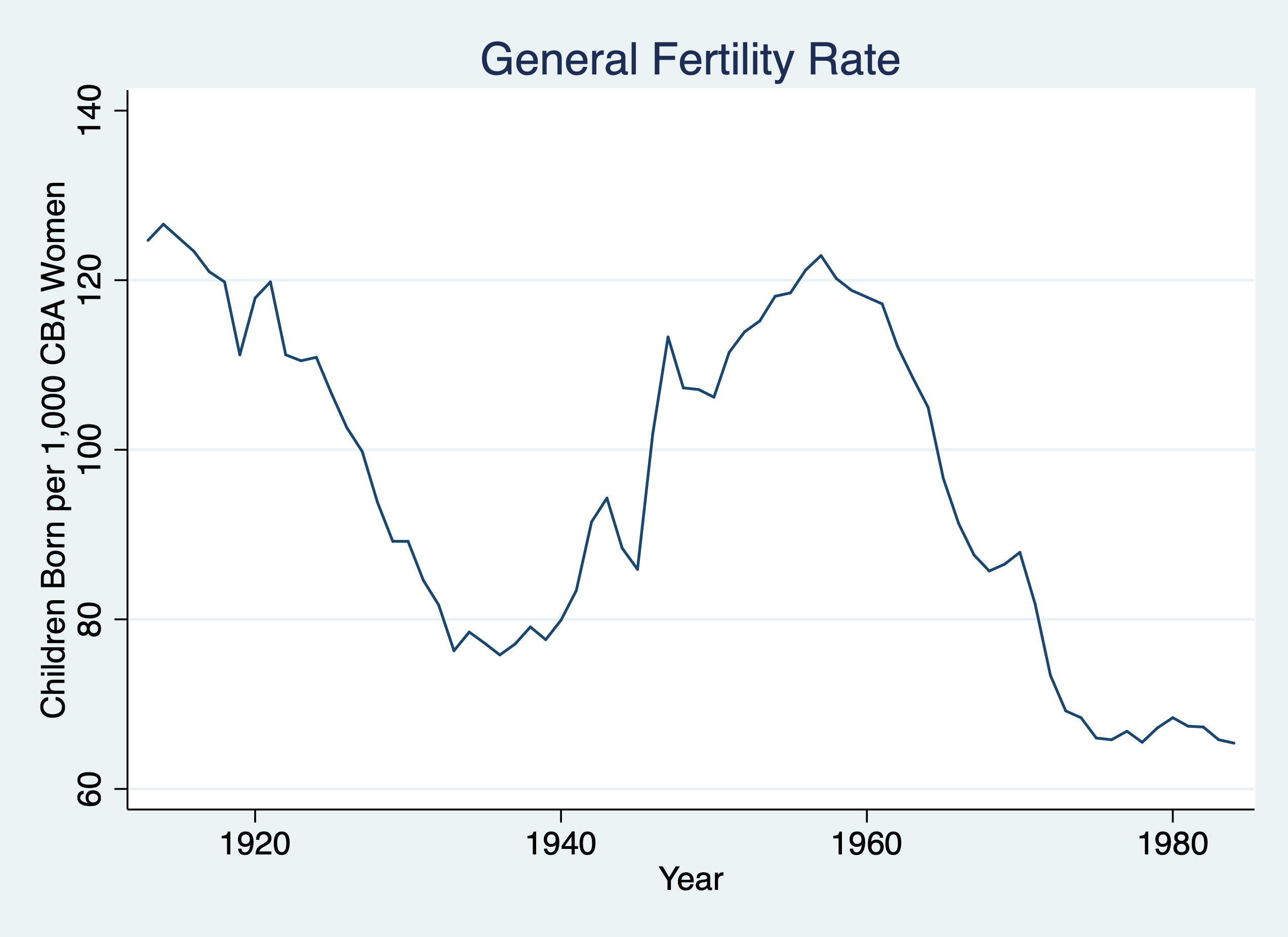
Estimate autocorrelation or estimate \(\hat{\rho}\)
      Source |       SS           df       MS      Number of obs   =        71
-------------+----------------------------------   F(1, 69)        =   1413.53
       Model |   25734.824         1   25734.824   Prob > F        =    0.0000
    Residual |  1256.21904        69  18.2060731   R-squared       =    0.9535
-------------+----------------------------------   Adj R-squared   =    0.9528
       Total |   26991.043        70  385.586329   Root MSE        =    4.2669

------------------------------------------------------------------------------
         gfr |      Coef.   Std. Err.      t    P>|t|     [95% Conf. Interval]
-------------+----------------------------------------------------------------
         gfr |
         L1. |   .9777202   .0260053    37.60   0.000      .925841    1.029599
             |
       _cons |   1.304937   2.548821     0.51   0.610    -3.779822    6.389695
------------------------------------------------------------------------------
Our result is rho-hat is 0.98, which is indicative of a unit root process. Under our TS assumptions our t statistics are invalid, but if we use a transformation using a first-difference process, we can relax those assumptions under the TSC assumptions. If our \(I(1)\) becomes \(I(0)\), then our TSC assumptions are potentially valid.
First Difference both dependent and independent
      Source |       SS           df       MS      Number of obs   =        71
-------------+----------------------------------   F(1, 69)        =      2.26
       Model |  40.3237206         1  40.3237206   Prob > F        =    0.1370
    Residual |  1229.25866        69  17.8153428   R-squared       =    0.0318
-------------+----------------------------------   Adj R-squared   =    0.0177
       Total |  1269.58238        70  18.1368911   Root MSE        =    4.2208

------------------------------------------------------------------------------
       D.gfr |      Coef.   Std. Err.      t    P>|t|     [95% Conf. Interval]
-------------+----------------------------------------------------------------
          pe |
         D1. |  -.0426776   .0283672    -1.50   0.137    -.0992686    .0139134
             |
       _cons |  -.7847796   .5020398    -1.56   0.123    -1.786322    .2167625
------------------------------------------------------------------------------
Our result is that the real value of the personal exemption is associated with a 0.043 decrease in fertility or a 23 dollar increase in the real value of the personal exemption is associated with a 1 child per capita (1,000 CBA Women). This is a bit unexpected, but still insignificant. Let’s add some lags.
First differnce with more than 1 lag
      Source |       SS           df       MS      Number of obs   =        69
-------------+----------------------------------   F(3, 65)        =      6.56
       Model |  293.259859         3  97.7532864   Prob > F        =    0.0006
    Residual |  968.199959        65   14.895384   R-squared       =    0.2325
-------------+----------------------------------   Adj R-squared   =    0.1971
       Total |  1261.45982        68  18.5508797   Root MSE        =    3.8595

------------------------------------------------------------------------------
       D.gfr |      Coef.   Std. Err.      t    P>|t|     [95% Conf. Interval]
-------------+----------------------------------------------------------------
          pe |
         D1. |  -.0362021   .0267737    -1.35   0.181     -.089673    .0172687
             |
        pe_1 |
         D1. |  -.0139706   .0275539    -0.51   0.614    -.0689997    .0410584
             |
        pe_2 |
         D1. |   .1099896   .0268797     4.09   0.000     .0563071    .1636721
             |
       _cons |  -.9636787   .4677599    -2.06   0.043     -1.89786   -.0294976
------------------------------------------------------------------------------
Our results show that increases in the current and prior period real value personal exemption is not statistically significant. However, a 1 dollar increase in the real value of personal exemption is associated two period prior is associated with an increase of .110 child per capita (or $9.1 increase is associated with an increase of 1 child per capita.
1.2 Wages and Productivity
\(I(1)\) process with the presence of a linear trend
We want to estimate the elasticity of hourly wage with respect to output per hour (or labor productivity).
\[ ln(hrwage_t)=\beta_0 + \beta_1 ln(outphr_t) + \beta_2 t + u_t \]
Set Time Series and estimate the contemporaneous model
cd "/Users/Sam/Desktop/Econ 645/Data/Wooldridge"
use earns.dta, clear
tsset year, yearly
reg lhrwage loutphr t
/Users/Sam/Desktop/Econ 645/Data/Wooldridge
time variable: year, 1947 to 1987
delta: 1 year
Source | SS df MS Number of obs = 41
-------------+---------------------------------- F(2, 38) = 641.22
Model | 1.04458064 2 .522290318 Prob > F = 0.0000
Residual | .030951776 38 .00081452 R-squared = 0.9712
-------------+---------------------------------- Adj R-squared = 0.9697
Total | 1.07553241 40 .02688831 Root MSE = .02854
------------------------------------------------------------------------------
lhrwage | Coef. Std. Err. t P>|t| [95% Conf. Interval]
-------------+----------------------------------------------------------------
loutphr | 1.639639 .0933471 17.56 0.000 1.450668 1.828611
t | -.01823 .0017482 -10.43 0.000 -.021769 -.0146909
_cons | -5.328454 .3744492 -14.23 0.000 -6.086487 -4.570421
------------------------------------------------------------------------------We estimate that the elasticity is very large, where a 1% increase in labor productivity (output per hour) is associated with a 1.64% increase in hourly wage. Let’s test for autocorrelation with accounting for the linear trend.
      Source |       SS           df       MS      Number of obs   =        40
-------------+----------------------------------   F(2, 37)        =   1595.37
       Model |  .921760671         2  .460880336   Prob > F        =    0.0000
    Residual |  .010688817        37  .000288887   R-squared       =    0.9885
-------------+----------------------------------   Adj R-squared   =    0.9879
       Total |  .932449488        39  .023908961   Root MSE        =      .017

------------------------------------------------------------------------------
     lhrwage |      Coef.   Std. Err.      t    P>|t|     [95% Conf. Interval]
-------------+----------------------------------------------------------------
     lhrwage |
         L1. |   .9842872   .0334331    29.44   0.000     .9165452    1.052029
             |
           t |  -.0009039   .0004732    -1.91   0.064    -.0018626    .0000548
       _cons |   .0544169   .0413998     1.31   0.197    -.0294671    .1383008
------------------------------------------------------------------------------
We have some evidence for a unit root process, so we’ll use the first-difference to transform the I(1) process into a I(0) process. We’ll no longer need the time trend
    twoway line lhrwage year, title("Natural Log of Hourly Wages") ytitle("Ln(Hourly Wage)") xtitle("Year")
    graph export "/Users/Sam/Desktop/Econ 645/Stata/week_11_hrwage1.png", replace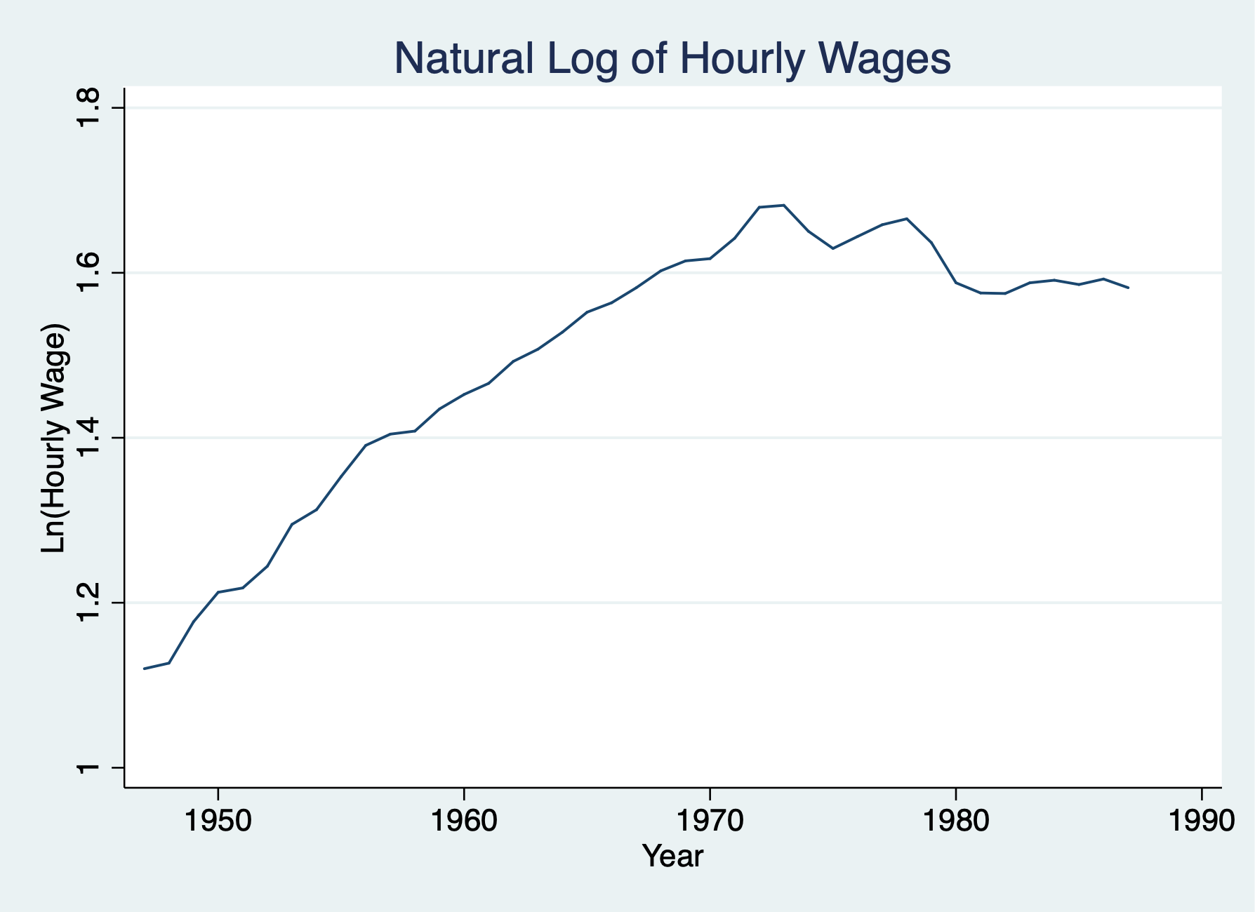
    twoway line d.lhrwage year, title("First-Difference in Ln(Hourly Wages)") ytitle("Delta Ln(Hourly Wage)") xtitle("Year")
    graph export "/Users/Sam/Desktop/Econ 645/Stata/week_11_hrwage2.png", replace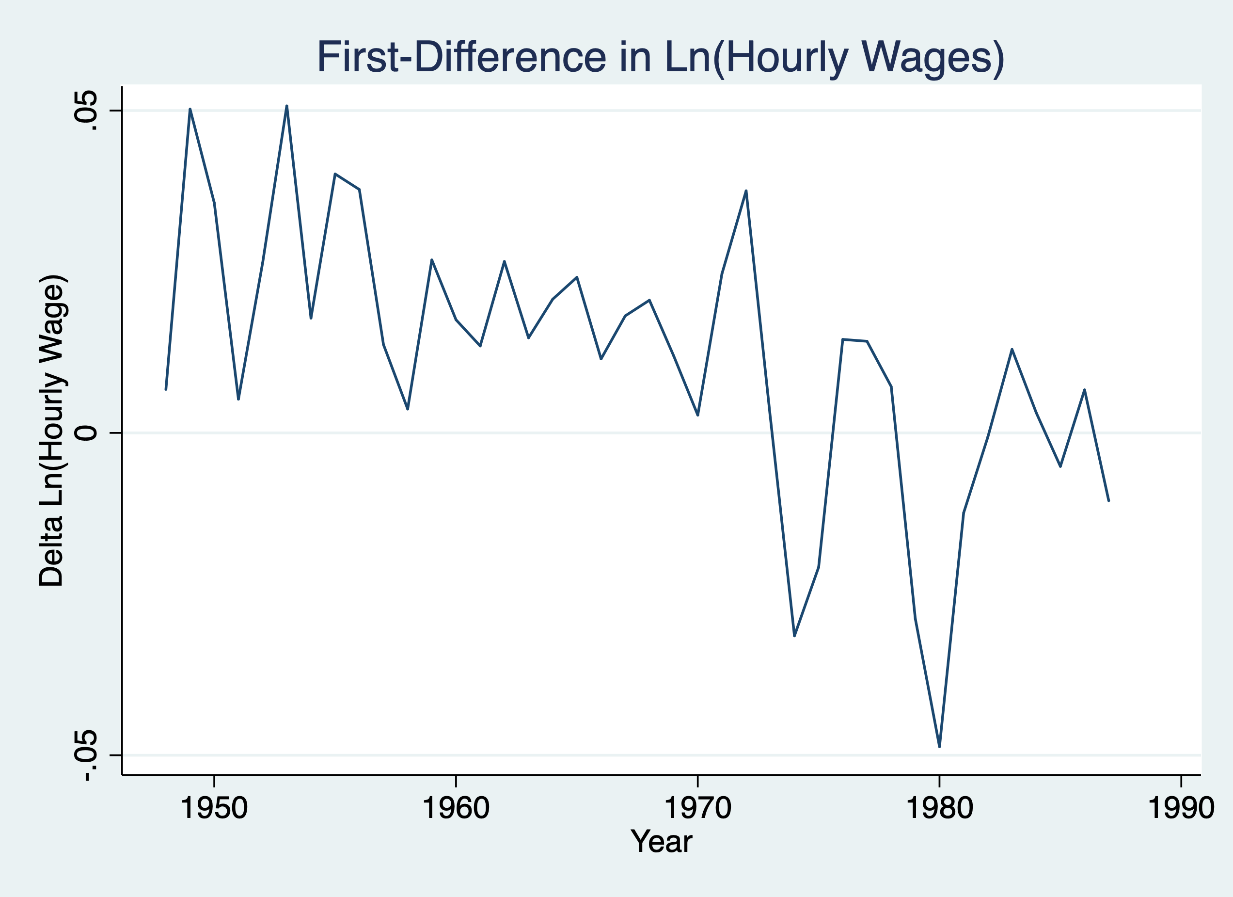
We’ll keep the trend based upon our prior graph
      Source |       SS           df       MS      Number of obs   =        40
-------------+----------------------------------   F(2, 37)        =     19.12
       Model |  .008727211         2  .004363605   Prob > F        =    0.0000
    Residual |  .008445792        37  .000228265   R-squared       =    0.5082
-------------+----------------------------------   Adj R-squared   =    0.4816
       Total |  .017173003        39  .000440333   Root MSE        =    .01511

------------------------------------------------------------------------------
   D.lhrwage |      Coef.   Std. Err.      t    P>|t|     [95% Conf. Interval]
-------------+----------------------------------------------------------------
     loutphr |
         D1. |   .5511404   .1733698     3.18   0.003     .1998598    .9024209
             |
           t |  -.0007637   .0002321    -3.29   0.002    -.0012339   -.0002935
       _cons |   .0176094   .0074784     2.35   0.024     .0024567    .0327622
------------------------------------------------------------------------------
Our transformed model shows that a 1% increase in output per hour is associated with a .55% increase in hourly wage.