Chapter 3 xtdidregress commmands
In addition to using xtreg or reg for estimating our \(\delta^{ATET}_{DD}\), we can use some built in Stata commands instead. These commands include xtdidregress and didregress.
For additional information we can use the help command.
Stata’s help page provides us with the following information:
For repeated cross-sections:
didregress (ovar omvarlist) (tvar[, continuous]) [if] [in] [weight], group(groupvars) [time(timevar) options]
For panel data:
xtdidregress (ovar omvarlist) (tvar[, continuous]) [if] [in] [weight], group(groupvars) [time(timevar) options]
Where 1. ovar is our outcome of interest 2. omvarlist is a list of our explanatory covariates 3. tvar is a binary indicating treatment status or a continuous indicating intensity of treatment 4. groupvars are categorical variables indicating treatment level, such as individual, state, etc. 5. timevar is our time variable, such as year
3.1 World Development Index
We will use the World Development Index to assess the impact of a trade policy in 2000 on total amount of trade (imports + exports) in millions of 2005 US dollars. These data are provided by Princeton.
/Users/Sam/Desktop/Econ 672/Data


Contains data from wdipol.dta
 Observations:         4,542
    Variables:            12                  26 Mar 2026 19:15
----------------------------------------------------------------------------------
Variable      Storage   Display    Value
    name         type    format    label      Variable label
----------------------------------------------------------------------------------
year            int     %10.0g                Year
country         str24   %24s                  Country Name
gdppc           double  %10.0g                 GDP per capita, PPP (constant 2005
                                                international $)
unempf          double  %10.0g                Unemployment, female (% of female
                                                labor force)
unempm          double  %10.0g                Unemployment, male (% of male labor
                                                force)
unemp           double  %10.0g                Unemployment, total (% of total
                                                labor force)
export          double  %10.0g                Exports of goods and services
                                                (constant 2005 US$)
import          double  %10.0g                Imports of goods and services
                                                (constant 2005 US$)
polity          byte    %8.0g                 polity (original)
polity2         byte    %8.0g                 polity2 (adjusted)
trade           float   %9.0g                 Imports + Exports
id              float   %9.0g                 group(country)
----------------------------------------------------------------------------------
Sorted by:
We will focus on years 1990 forward.
(1,136 observations deleted)

      Exports of goods and services (constant 2005 US$)
-------------------------------------------------------------
      Percentiles      Smallest
 1%     91.64278       45.02022
 5%     245.0359       48.62297
10%     543.8475       52.79048       Obs               2,814
25%     2094.341       53.24336       Sum of wgt.       2,814

50%     8836.828                      Mean           75432.49
                        Largest       Std. dev.      182677.6
75%     57261.36        1649300
90%     198699.2        1665600       Variance       3.34e+10
95%     399759.2        1677840       Skewness       4.764539
99%      1036798        1776900       Kurtosis       31.56892

      Imports of goods and services (constant 2005 US$)
-------------------------------------------------------------
      Percentiles      Smallest
 1%     264.6554       94.23958
 5%     538.7271       110.3702
10%     1031.108       129.2793       Obs               2,814
25%     2514.115       135.4336       Sum of wgt.       2,814

50%      10218.4                      Mean           74643.16
                        Largest       Std. dev.        194233
75%     56131.35        2144000
90%     182048.5        2151500       Variance       3.77e+10
95%     371224.2        2184900       Skewness       5.811369
99%       943900        2203200       Kurtosis       47.77702

                      Imports + Exports
-------------------------------------------------------------
      Percentiles      Smallest
 1%     414.4894       139.2598
 5%     828.4978       166.8271
10%      1613.88       183.3966       Obs               2,814
25%     4867.792       193.1237       Sum of wgt.       2,814

50%     19421.02                      Mean           150075.7
                        Largest       Std. dev.      374324.7
75%     115498.2        3750800
90%     382896.8        3757600       Variance       1.40e+11
95%     759593.4        3793300       Skewness       5.158498
99%      2001955        3961800       Kurtosis       37.13028
Looking at combined imports and exports, the median amount of trade is 19.4 billion 2005 US dollars.
Now, we set our post period at 2000 or later. An indicator for when trade relations were normalized between the U.S. and China and China’s ascension into the World Trade Organization (WTO).
Next we will assign the treatment countries, which are the following western countries: Australia, Austria, Belgium, Canada, Denmark, Finland, France, Germany, Greece, Ireland, Italy, Luxembourg, Netherlands, New Zealand, Norway, Portugal, Spain, Sweden, Switzerland, United Kingdom, and United States.
gen treatment = 0
replace treatment = 1 if country == "Australia" | country == "Austria" | country == "Belgium" | country == "Canada" | country == "Denmark" | country == "Finland" | country == "France" | country == "Germany" | country == "Greece" | country == "Ireland" | country == "Italy" | country == "Luxembourg" | country == "Netherlands" | country == "New Zealand" | country == "Norway" | country == "Portugal" | country == "Spain" |country == "Sweden" | country == "Switzerland" | country == "United Kingdom" | country == "United States"
Next, we will set up the difference-in-differences interaction.
Now we need to establish our panel, but we need to use the encode command on countries so we can use the xtset command.
*Encode country
encode country, gen(countrynum)

*Set Panel
sort countrynum year
xtset countrynum year
Panel variable: countrynum (unbalanced)
Time variable: year, 1990 to 2012, but with a gap
Delta: 1 unitOur panel is unbalanced, which means we do have gaps among some of the countries.
We will first start with our tried and true method with xtreg and use the fe option, and we will cluster our standard errors at the unit of observation level.
Fixed-effects (within) regression               Number of obs     =      2,814
Group variable: countrynum                      Number of groups  =        153

R-squared:                                      Obs per group:
     Within  = 0.2476                                         min =          1
     Between = 0.2331                                         avg =       18.4
     Overall = 0.1877                                         max =         23

                                                F(23, 152)        =       2.88
corr(u_i, Xb) = 0.2187                          Prob > F          =     0.0001

                           (Std. err. adjusted for 153 clusters in countrynum)
------------------------------------------------------------------------------
             |               Robust
       trade | Coefficient  std. err.      t    P>|t|     [95% conf. interval]
-------------+----------------------------------------------------------------
  treat_post |   254619.5   84665.83     3.01   0.003     87345.69    421893.2
             |
        year |
       1991  |   11417.79   3273.274     3.49   0.001     4950.798    17884.77
       1992  |   14691.17   4183.539     3.51   0.001     6425.782    22956.57
       1993  |   17823.51   5089.347     3.50   0.001     7768.513     27878.5
       1994  |   27212.01   6768.259     4.02   0.000     13840.01    40584.02
       1995  |   36908.65   8577.682     4.30   0.000     19961.77    53855.52
       1996  |    43697.3   9997.622     4.37   0.000     23945.06    63449.54
       1997  |   53882.39   12313.33     4.38   0.000     29555.02    78209.75
       1998  |   60352.96   13818.67     4.37   0.000      33051.5    87654.42
       1999  |   67276.08   15777.22     4.26   0.000     36105.13    98447.04
       2000  |   43940.78   12961.89     3.39   0.001     18332.06     69549.5
       2001  |   45574.41   13023.31     3.50   0.001     19844.34    71304.49
       2002  |   50357.95    14195.9     3.55   0.001     22311.21     78404.7
       2003  |   58200.38    16052.8     3.63   0.000     26484.97    89915.79
       2004  |   74493.25   18905.12     3.94   0.000     37142.52      111844
       2005  |    87670.9   21325.73     4.11   0.000     45537.78      129804
       2006  |   104994.9   24623.44     4.26   0.000     56346.51    153643.3
       2007  |   121106.3   28005.54     4.32   0.000     65775.88    176436.6
       2008  |   128370.5   29721.71     4.32   0.000     69649.48    187091.5
       2009  |   104644.4   27073.14     3.87   0.000     51156.19    158132.7
       2010  |   131099.8   33071.58     3.96   0.000     65760.48    196439.1
       2011  |   149272.6   37479.36     3.98   0.000     75224.91    223320.4
       2012  |   129456.8   24816.73     5.22   0.000     80426.54    178487.1
             |
       _cons |   56946.96   18846.82     3.02   0.003     19711.41    94182.51
-------------+----------------------------------------------------------------
     sigma_u |  295226.32
     sigma_e |   132684.6
         rho |  .83195335   (fraction of variance due to u_i)
------------------------------------------------------------------------------
Our difference-in-difference estimator indicates that the change in trade policy increased total trade by 255 billion 2005 US dollars, which is statistically significant at the 1% level.
To visualize our parallel trends, we need to use egen to get the mean outcome by year for treatment and comparison groups. Next, we will visually inspect the parallel trends assumption with twoway line charts.
bysort year treatment: egen mean_trade = mean(trade)

twoway line mean_trade year if treatment == 0, sort || ///
       line mean_trade year if treatment == 1, sort lpattern (dash) ///
       legend(label(1 "Control") label(2 "Treated")) ///
       xline(2000) title("Check Parallel Trends Assumption")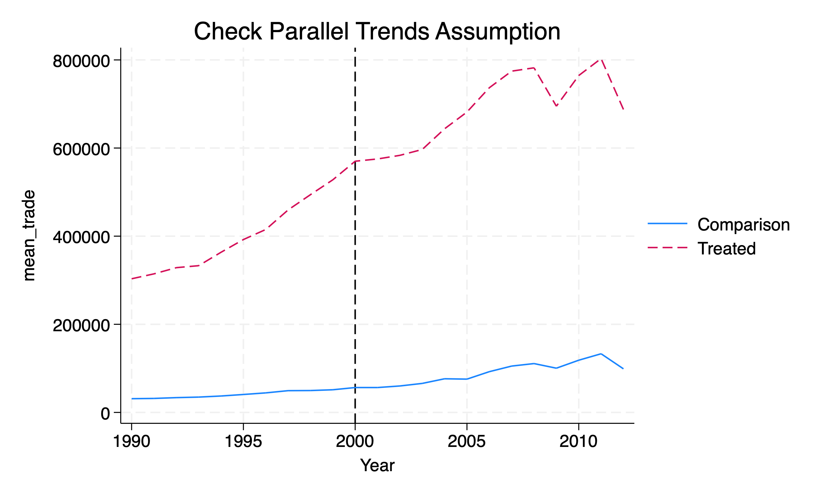
3.2 xtdidregress
We have other commands for estimating difference-in-differences, such as the xtdidregress and didregress commands. These commands will estimate our \(\delta^{ATET}_{DD}\) of interest.
Why should we use this command? They provide helpful post-estimation commands for testing the parallel trends assumption!
Treatment and time information

Time variable: year
Control:       treat_post = 0
Treatment:     treat_post = 1
-----------------------------------
             |   Control  Treatment
-------------+---------------------
Group        |
  countrynum |       132         21
-------------+---------------------
Time         |
     Minimum |      1990       2000
     Maximum |      2006       2000
-----------------------------------

Difference-in-differences regression                     Number of obs = 2,814
Data type: Longitudinal

                           (Std. err. adjusted for 153 clusters in countrynum)
------------------------------------------------------------------------------
             |               Robust
       trade | Coefficient  std. err.      t    P>|t|     [95% conf. interval]
-------------+----------------------------------------------------------------
ATET         |
  treat_post |
   (1 vs 0)  |   254619.5   84665.83     3.01   0.003     87345.69    421893.2
------------------------------------------------------------------------------
Note: ATET estimate adjusted for panel effects and time effects.
Note: Treatment occurs at different times.
We get the same result, such that trade increases $254,619.5 millions or 255 billion 2005 US dollars
We can also add some covariates in case the parallel trends is conditional on controlling for covariates.
Treatment and time information

Time variable: year
Control:       treat_post = 0
Treatment:     treat_post = 1
-----------------------------------
             |   Control  Treatment
-------------+---------------------
Group        |
  countrynum |       132         21
-------------+---------------------
Time         |
     Minimum |      1990       2000
     Maximum |      2006       2000
-----------------------------------

Difference-in-differences regression                     Number of obs = 2,804
Data type: Longitudinal

                           (Std. err. adjusted for 153 clusters in countrynum)
------------------------------------------------------------------------------
             |               Robust
       trade | Coefficient  std. err.      t    P>|t|     [95% conf. interval]
-------------+----------------------------------------------------------------
ATET         |
  treat_post |
   (1 vs 0)  |   253104.1   85410.71     2.96   0.004     84358.69    421849.5
------------------------------------------------------------------------------
Note: ATET estimate adjusted for covariates, panel effects, and time effects.
Note: Treatment occurs at different times.
Our estimate is little change after controlling for unemployment and political system of the country. Our estimate is \(\hat{\delta}^{ATET}_{DD}=\$253B\).