Chapter 4 Postestimation Command
The question remains if our parallel trends assummption holds. We visually inspected the parallel trends assumption with a graph, but we did not test any null hypotheses. With the xtdidregress and didregress commands we have two helpful commands: estat ptrends and estat trendplots.
4.1 estat ptrends
Let’s test the null hypothesis that the trends between treatment and comparison are the same. We will use the diff-in-diff without covariates first
Parallel-trends test (pretreatment time period)
H0: Linear trends are parallel

F(1, 152) =   9.09
 Prob > F = 0.0030
Our \(F\)-statistic is \(9.09\) and we reject the null hypothesis at the 1% level. Now let’s add the covariates to see if parallel trends are conditional on additional covariates of unemployment and political system.
Parallel-trends test (pretreatment time period)
H0: Linear trends are parallel

F(1, 152) =   8.85
 Prob > F = 0.0034
Our \(F\)-statistic barely changes and we reject the null hypothesis at the 1% level.
4.2 estat trendsplot
Even though we reject the null hypothesis at the 1% level, we can still provide a visualization that is easier to implement than our twoway line graph above. With estat trendsplot, the syntax is more concise and less likely to have an operator error. With the twoway line command, we need to make sure to graph both treatment and comparison lines.
We will compare the parallel trends with and without covariates. The command is the same regardless if we have covariates or not.
quietly xtdidregress (trade) (treat_post), group(countrynum) time(year)
estat trendplots, ytitle(Trade in millions of 2005 USD) xlabel(1990(2)2012)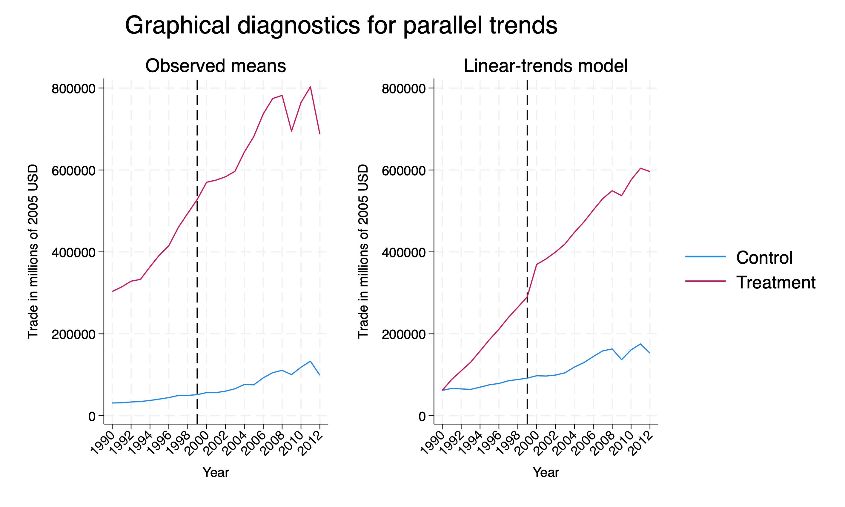
We can clearly see that the parallel trend assumption does not hold. This visually confirms what we saw with out \(F\)-test.
Next, we will add covariates.
quietly xtdidregress (trade) (treat_post), group(countrynum) time(year)
estat trendplots, ytitle(Trade in millions of 2005 USD) xlabel(1990(2)2012)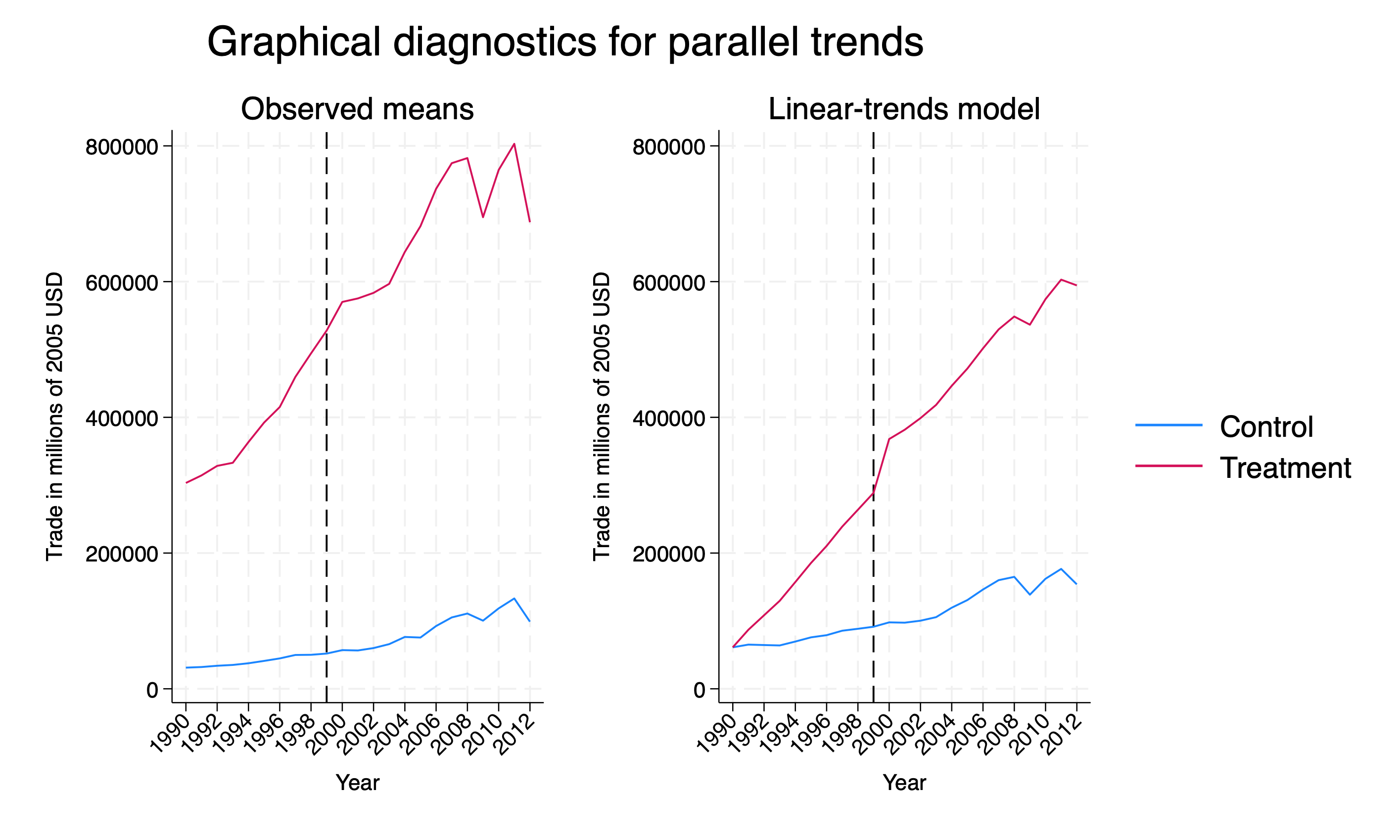
Again, we clearly see that the parallel trends assumption does not hold even if we add covariates.