. clear

. set more off
Set Working Directory
. cd "/Users/Sam/Desktop/Econ 645/Data/Wooldridge"
/Users/Sam/Desktop/Econ 645/Data/Wooldridge
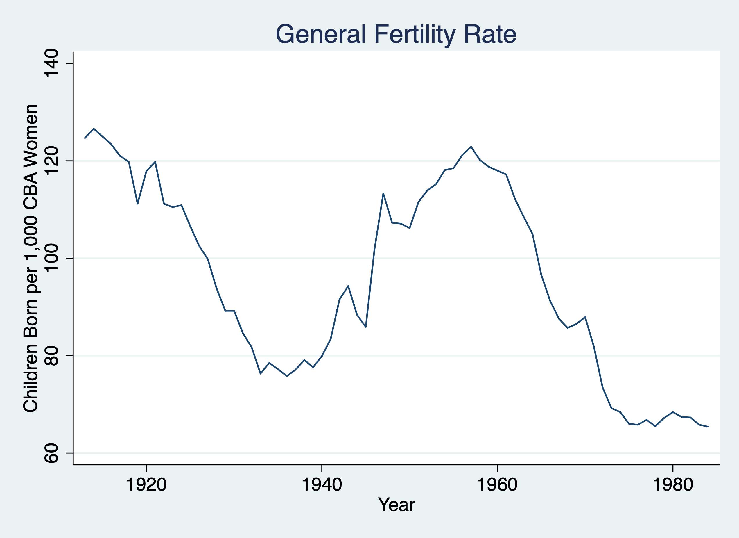
. use fertil3.dta, clear
Set Time Series
. tsset year
        time variable:  year, 1913 to 1984
                delta:  1 unit
. twoway line gfr year, title("General Fertility Rate") ytitle("Children Born per 1,000 CBA Women") xtitle("Year")

. graph export "/Users/Sam/Desktop/Econ 645/Stata/week_11_i1.png", replace
(file /Users/Sam/Desktop/Econ 645/Stata/week_11_i1.png written in PNG format)
Estimate autocorrelation or estimate rho-hat
. reg gfr l.gfr

      Source │       SS           df       MS      Number of obs   =        71
─────────────┼──────────────────────────────────   F(1, 69)        =   1413.53
       Model │   25734.824         1   25734.824   Prob > F        =    0.0000
    Residual │  1256.21904        69  18.2060731   R-squared       =    0.9535
─────────────┼──────────────────────────────────   Adj R-squared   =    0.9528
       Total │   26991.043        70  385.586329   Root MSE        =    4.2669

─────────────┬────────────────────────────────────────────────────────────────
         gfr │      Coef.   Std. Err.      t    P>|t|     [95% Conf. Interval]
─────────────┼────────────────────────────────────────────────────────────────
         gfr │
         L1. │   .9777202   .0260053    37.60   0.000      .925841    1.029599
             │
       _cons │   1.304937   2.548821     0.51   0.610    -3.779822    6.389695
─────────────┴────────────────────────────────────────────────────────────────
Our result is rho-hat is 0.98, which is indicative of a unit root process. Under our TS assumptions our t statistics are invalid, but if we use a transformation using a first-difference process, we can relax those assumptions under the TSC assumptions. If our I(1) becomes I(0), then our TSC assumptions are potentially valid.
First Difference both dependent and independent
. reg d.gfr d.pe if year < 1985

      Source │       SS           df       MS      Number of obs   =        71
─────────────┼──────────────────────────────────   F(1, 69)        =      2.26
       Model │  40.3237206         1  40.3237206   Prob > F        =    0.1370
    Residual │  1229.25866        69  17.8153428   R-squared       =    0.0318
─────────────┼──────────────────────────────────   Adj R-squared   =    0.0177
       Total │  1269.58238        70  18.1368911   Root MSE        =    4.2208

─────────────┬────────────────────────────────────────────────────────────────
       D.gfr │      Coef.   Std. Err.      t    P>|t|     [95% Conf. Interval]
─────────────┼────────────────────────────────────────────────────────────────
          pe │
         D1. │  -.0426776   .0283672    -1.50   0.137    -.0992686    .0139134
             │
       _cons │  -.7847796   .5020398    -1.56   0.123    -1.786322    .2167625
─────────────┴────────────────────────────────────────────────────────────────
Our result is that the real value of the personal exemption is associated with a 0.043 decrease in fertility or a 23 dollar increase in the real value of the personal exemption is associated with a 1 child per capita (1,000 CBA Women). This is a bit unexpected, but still insignificant. Let’s add some lags.
First differnce with more than 1 lag
. reg d.gfr d.pe d.pe_1 d.pe_2 if year < 1985

      Source │       SS           df       MS      Number of obs   =        69
─────────────┼──────────────────────────────────   F(3, 65)        =      6.56
       Model │  293.259859         3  97.7532864   Prob > F        =    0.0006
    Residual │  968.199959        65   14.895384   R-squared       =    0.2325
─────────────┼──────────────────────────────────   Adj R-squared   =    0.1971
       Total │  1261.45982        68  18.5508797   Root MSE        =    3.8595

─────────────┬────────────────────────────────────────────────────────────────
       D.gfr │      Coef.   Std. Err.      t    P>|t|     [95% Conf. Interval]
─────────────┼────────────────────────────────────────────────────────────────
          pe │
         D1. │  -.0362021   .0267737    -1.35   0.181     -.089673    .0172687
             │
        pe_1 │
         D1. │  -.0139706   .0275539    -0.51   0.614    -.0689997    .0410584
             │
        pe_2 │
         D1. │   .1099896   .0268797     4.09   0.000     .0563071    .1636721
             │
       _cons │  -.9636787   .4677599    -2.06   0.043     -1.89786   -.0294976
─────────────┴────────────────────────────────────────────────────────────────
Our results show that increases in the current and prior period real value personal exemption is not statistically significant. However, a 1 dollar increase in the real value of personal exemption is associated two period prior is associated with an increase of .110 child per capita (or $9.1 increase is associated with an increase of 1 child per capita.
I(1) process with the presence of a linear trend
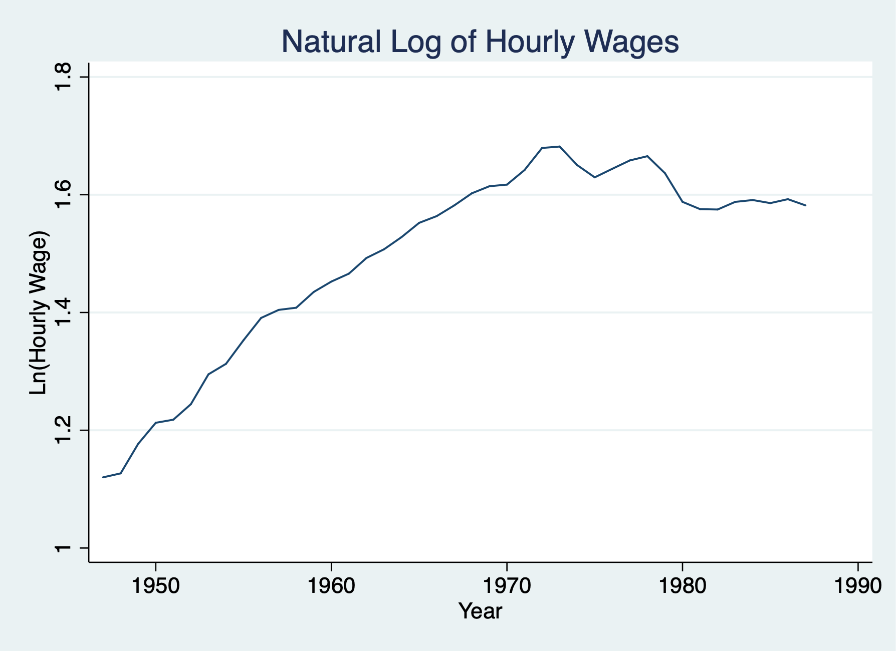
. use earns.dta, clear
Set Time Series
. tsset year, yearly
        time variable:  year, 1947 to 1987
                delta:  1 year
We want to estimate the elasticity of hourly wage with respect to output per hour (or labor productivity). \[ ln(hrwage_t)=\beta_0 + \beta_1 ln(outphr_t) + \beta_2 t + u_t \]
We estimate the contemporaneous model
. reg lhrwage loutphr t

      Source │       SS           df       MS      Number of obs   =        41
─────────────┼──────────────────────────────────   F(2, 38)        =    641.22
       Model │  1.04458064         2  .522290318   Prob > F        =    0.0000
    Residual │  .030951776        38   .00081452   R-squared       =    0.9712
─────────────┼──────────────────────────────────   Adj R-squared   =    0.9697
       Total │  1.07553241        40   .02688831   Root MSE        =    .02854

─────────────┬────────────────────────────────────────────────────────────────
     lhrwage │      Coef.   Std. Err.      t    P>|t|     [95% Conf. Interval]
─────────────┼────────────────────────────────────────────────────────────────
     loutphr │   1.639639   .0933471    17.56   0.000     1.450668    1.828611
           t │    -.01823   .0017482   -10.43   0.000     -.021769   -.0146909
       _cons │  -5.328454   .3744492   -14.23   0.000    -6.086487   -4.570421
─────────────┴────────────────────────────────────────────────────────────────
We estimate that the elasticity is very large, where a 1% increase in labor productivity (output per hour) is associated with a 1.64% increase in hourly wage. Let’s test for autocorrelation with accounting for the linear trend.
. reg lhrwage l.lhrwage t

      Source │       SS           df       MS      Number of obs   =        40
─────────────┼──────────────────────────────────   F(2, 37)        =   1595.37
       Model │  .921760671         2  .460880336   Prob > F        =    0.0000
    Residual │  .010688817        37  .000288887   R-squared       =    0.9885
─────────────┼──────────────────────────────────   Adj R-squared   =    0.9879
       Total │  .932449488        39  .023908961   Root MSE        =      .017

─────────────┬────────────────────────────────────────────────────────────────
     lhrwage │      Coef.   Std. Err.      t    P>|t|     [95% Conf. Interval]
─────────────┼────────────────────────────────────────────────────────────────
     lhrwage │
         L1. │   .9842872   .0334331    29.44   0.000     .9165452    1.052029
             │
           t │  -.0009039   .0004732    -1.91   0.064    -.0018626    .0000548
       _cons │   .0544169   .0413998     1.31   0.197    -.0294671    .1383008
─────────────┴────────────────────────────────────────────────────────────────
We have some evidence for a unit root process, so we’ll use the first-difference to transform the I(1) process into a I(0) process. We’ll no longer need the time trend
. twoway line lhrwage year, title("Natural Log of Hourly Wages") ytitle("Ln(Hourly Wage)") xtitle("Year")

. graph export "/Users/Sam/Desktop/Econ 645/Stata/week_11_hrwage1.png", replace
(file /Users/Sam/Desktop/Econ 645/Stata/week_11_hrwage1.png written in PNG format)
. twoway line d.lhrwage year, title("First-Difference in Ln(Hourly Wages)") ytitle("Delta Ln(Hourly Wage)") xtitle(
> "Year")

. graph export "/Users/Sam/Desktop/Econ 645/Stata/week_11_hrwage2.png", replace
(file /Users/Sam/Desktop/Econ 645/Stata/week_11_hrwage2.png written in PNG format)
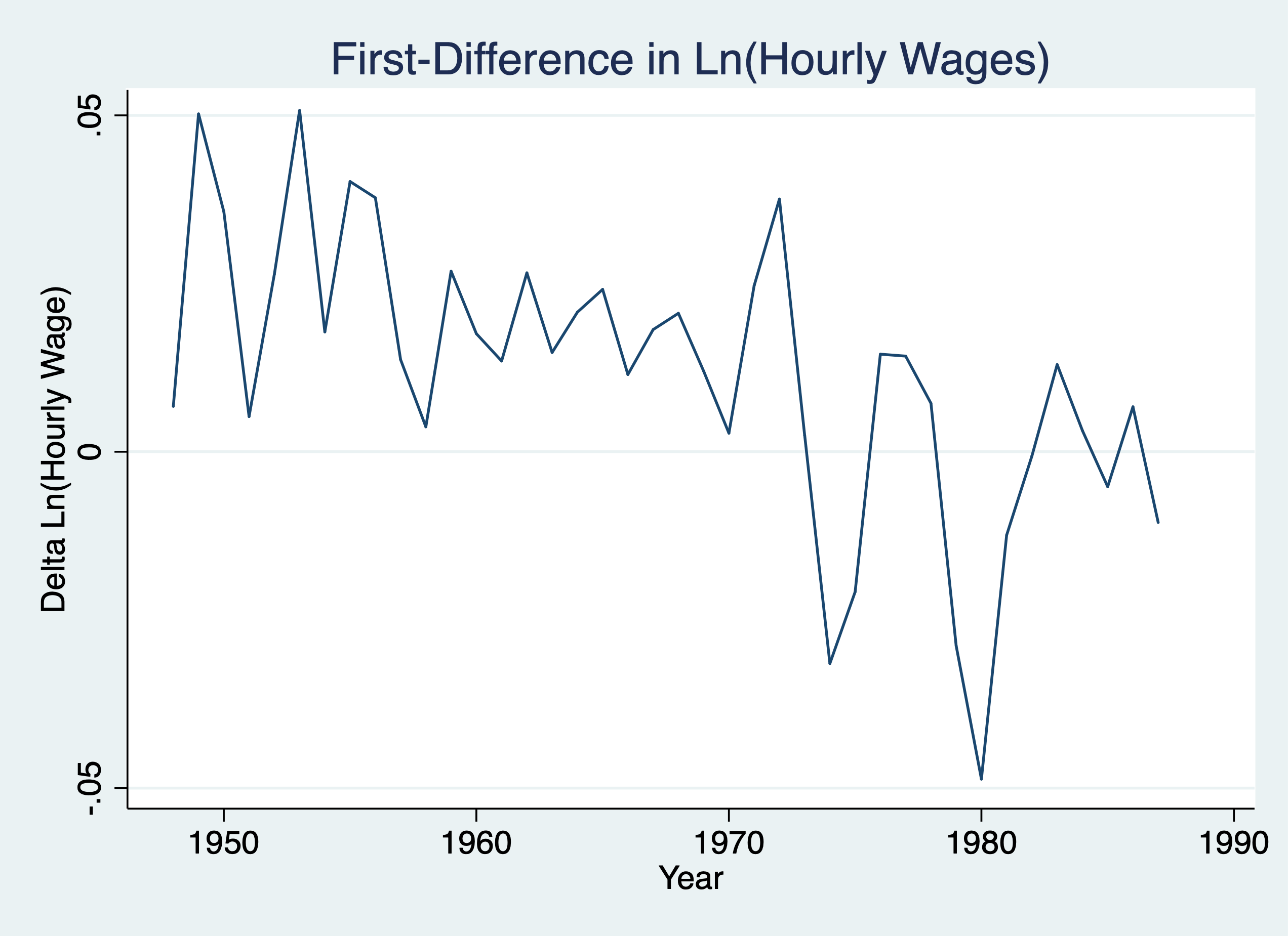
We’ll keep the trend based upon our prior graph
. reg d.lhrwage d.loutphr t

      Source │       SS           df       MS      Number of obs   =        40
─────────────┼──────────────────────────────────   F(2, 37)        =     19.12
       Model │  .008727211         2  .004363605   Prob > F        =    0.0000
    Residual │  .008445792        37  .000228265   R-squared       =    0.5082
─────────────┼──────────────────────────────────   Adj R-squared   =    0.4816
       Total │  .017173003        39  .000440333   Root MSE        =    .01511

─────────────┬────────────────────────────────────────────────────────────────
   D.lhrwage │      Coef.   Std. Err.      t    P>|t|     [95% Conf. Interval]
─────────────┼────────────────────────────────────────────────────────────────
     loutphr │
         D1. │   .5511404   .1733698     3.18   0.003     .1998598    .9024209
             │
           t │  -.0007637   .0002321    -3.29   0.002    -.0012339   -.0002935
       _cons │   .0176094   .0074784     2.35   0.024     .0024567    .0327622
─────────────┴────────────────────────────────────────────────────────────────
Our transformed model shows that a 1% increase in output per hour is associated with a .55% increase in hourly wage.
. use fertil3.dta
Set Time Series
. tsset year, yearly
        time variable:  year, 1913 to 1984
                delta:  1 year
We’ll estimate a Finite Distributed Lag model for the first difference of general fertility onto the first difference of personal exemptions. If our model is dynamically complete, then no additional lags of gfr or pe are needed.
Our First-difference model with one lag of pe
. reg d.gfr d.pe d.pe_1 if year < 1985

      Source │       SS           df       MS      Number of obs   =        70
─────────────┼──────────────────────────────────   F(2, 67)        =      1.20
       Model │  43.7985353         2  21.8992676   Prob > F        =    0.3063
    Residual │  1218.19557        67  18.1820235   R-squared       =    0.0347
─────────────┼──────────────────────────────────   Adj R-squared   =    0.0059
       Total │  1261.99411        69  18.2897697   Root MSE        =     4.264

─────────────┬────────────────────────────────────────────────────────────────
       D.gfr │      Coef.   Std. Err.      t    P>|t|     [95% Conf. Interval]
─────────────┼────────────────────────────────────────────────────────────────
          pe │
         D1. │  -.0456497   .0294689    -1.55   0.126    -.1044699    .0131704
             │
        pe_1 │
         D1. │   .0134149   .0295326     0.45   0.651    -.0455324    .0723623
             │
       _cons │  -.8372962   .5117337    -1.64   0.106    -1.858721    .1841286
─────────────┴────────────────────────────────────────────────────────────────
Is this dynamically complete? Let’s add a second lag of pe
. reg d.gfr d.pe d.pe_1 d.pe_2 if year < 1985

      Source │       SS           df       MS      Number of obs   =        69
─────────────┼──────────────────────────────────   F(3, 65)        =      6.56
       Model │  293.259859         3  97.7532864   Prob > F        =    0.0006
    Residual │  968.199959        65   14.895384   R-squared       =    0.2325
─────────────┼──────────────────────────────────   Adj R-squared   =    0.1971
       Total │  1261.45982        68  18.5508797   Root MSE        =    3.8595

─────────────┬────────────────────────────────────────────────────────────────
       D.gfr │      Coef.   Std. Err.      t    P>|t|     [95% Conf. Interval]
─────────────┼────────────────────────────────────────────────────────────────
          pe │
         D1. │  -.0362021   .0267737    -1.35   0.181     -.089673    .0172687
             │
        pe_1 │
         D1. │  -.0139706   .0275539    -0.51   0.614    -.0689997    .0410584
             │
        pe_2 │
         D1. │   .1099896   .0268797     4.09   0.000     .0563071    .1636721
             │
       _cons │  -.9636787   .4677599    -2.06   0.043     -1.89786   -.0294976
─────────────┴────────────────────────────────────────────────────────────────
Add lag of d.gfr and see it wasn’t dynamically complete
. reg d.gfr d.gfr_1 d.pe d.pe_1 d.pe_2 if year < 1985

      Source │       SS           df       MS      Number of obs   =        69
─────────────┼──────────────────────────────────   F(4, 64)        =      7.46
       Model │  401.286162         4   100.32154   Prob > F        =    0.0001
    Residual │  860.173657        64  13.4402134   R-squared       =    0.3181
─────────────┼──────────────────────────────────   Adj R-squared   =    0.2755
       Total │  1261.45982        68  18.5508797   Root MSE        =    3.6661

─────────────┬────────────────────────────────────────────────────────────────
       D.gfr │      Coef.   Std. Err.      t    P>|t|     [95% Conf. Interval]
─────────────┼────────────────────────────────────────────────────────────────
       gfr_1 │
         D1. │   .3002422   .1059034     2.84   0.006     .0886758    .5118086
             │
          pe │
         D1. │  -.0454721   .0256417    -1.77   0.081    -.0966972     .005753
             │
        pe_1 │
         D1. │    .002064   .0267776     0.08   0.939    -.0514303    .0555584
             │
        pe_2 │
         D1. │   .1051346   .0255904     4.11   0.000      .054012    .1562572
             │
       _cons │  -.7021594   .4537988    -1.55   0.127    -1.608727    .2044079
─────────────┴────────────────────────────────────────────────────────────────
We’ll use our t-test for serial correlation with strictly exogenous regressors under the assumption that our regressors are exogenous.
. use phillips.dta, clear
Set Time Series
. tsset year, yearly
        time variable:  year, 1948 to 2003
                delta:  1 year
We estimated a static Phillips Curve and an augmented Phillips Curve last week. We’ll retest the models for serial correlation.
Test for serial correlation in Static Model Noticeable serial correlation
. reg inf unem if year < 1997

      Source │       SS           df       MS      Number of obs   =        49
─────────────┼──────────────────────────────────   F(1, 47)        =      2.62
       Model │  25.6369575         1  25.6369575   Prob > F        =    0.1125
    Residual │   460.61979        47  9.80042107   R-squared       =    0.0527
─────────────┼──────────────────────────────────   Adj R-squared   =    0.0326
       Total │  486.256748        48  10.1303489   Root MSE        =    3.1306

─────────────┬────────────────────────────────────────────────────────────────
         inf │      Coef.   Std. Err.      t    P>|t|     [95% Conf. Interval]
─────────────┼────────────────────────────────────────────────────────────────
        unem │   .4676257   .2891262     1.62   0.112    -.1140213    1.049273
       _cons │    1.42361   1.719015     0.83   0.412    -2.034602    4.881822
─────────────┴────────────────────────────────────────────────────────────────
Breusch-Godfrey Test
. estat bgodfrey

Breusch-Godfrey LM test for autocorrelation
─────────────┬─────────────────────────────────────────────────────────────
    lags(p)  │          chi2               df                 Prob > chi2
─────────────┼─────────────────────────────────────────────────────────────
       1     │         18.472               1                   0.0000
─────────────┴─────────────────────────────────────────────────────────────
                        H0: no serial correlation
Simple AR(1) test
. predict u, resid
. reg u l.u, noconst

      Source │       SS           df       MS      Number of obs   =        55
─────────────┼──────────────────────────────────   F(1, 54)        =     29.61
       Model │  161.010846         1  161.010846   Prob > F        =    0.0000
    Residual │  293.652171        54  5.43800317   R-squared       =    0.3541
─────────────┼──────────────────────────────────   Adj R-squared   =    0.3422
       Total │  454.663017        55  8.26660031   Root MSE        =     2.332

─────────────┬────────────────────────────────────────────────────────────────
           u │      Coef.   Std. Err.      t    P>|t|     [95% Conf. Interval]
─────────────┼────────────────────────────────────────────────────────────────
           u │
         L1. │   .5822453   .1070035     5.44   0.000     .3677161    .7967745
─────────────┴────────────────────────────────────────────────────────────────
Test for serial correlation in Augmented Serial correlation is removed with the first-difference in inflation
. reg d.inf unem if year < 1997

      Source │       SS           df       MS      Number of obs   =        48
─────────────┼──────────────────────────────────   F(1, 46)        =      5.56
       Model │  33.3829996         1  33.3829996   Prob > F        =    0.0227
    Residual │  276.305138        46  6.00663344   R-squared       =    0.1078
─────────────┼──────────────────────────────────   Adj R-squared   =    0.0884
       Total │  309.688138        47  6.58910932   Root MSE        =    2.4508

─────────────┬────────────────────────────────────────────────────────────────
       D.inf │      Coef.   Std. Err.      t    P>|t|     [95% Conf. Interval]
─────────────┼────────────────────────────────────────────────────────────────
        unem │  -.5425869   .2301559    -2.36   0.023    -1.005867    -.079307
       _cons │   3.030581    1.37681     2.20   0.033      .259206    5.801955
─────────────┴────────────────────────────────────────────────────────────────

. predict u2, resid
(1 missing value generated)
Breusch-Godfrey Test
. estat bgodfrey

Breusch-Godfrey LM test for autocorrelation
─────────────┬─────────────────────────────────────────────────────────────
    lags(p)  │          chi2               df                 Prob > chi2
─────────────┼─────────────────────────────────────────────────────────────
       1     │          0.062               1                   0.8039
─────────────┴─────────────────────────────────────────────────────────────
                        H0: no serial correlation
Durban-Watson Test
. estat dwatson

Durbin-Watson d-statistic(  2,    48) =  1.769648
\[ d_L = 1.503 \] \[ d_U = 1.585 \] \[ 1.769648 > 1.585 \] We fail to reject the null hypothesis.
AR(1) Test
. reg u2 l.u2, noconst

      Source │       SS           df       MS      Number of obs   =        54
─────────────┼──────────────────────────────────   F(1, 53)        =      0.07
       Model │  .267251656         1  .267251656   Prob > F        =    0.7905
    Residual │  198.724905        53  3.74952651   R-squared       =    0.0013
─────────────┼──────────────────────────────────   Adj R-squared   =   -0.0175
       Total │  198.992157        54  3.68503994   Root MSE        =    1.9364

─────────────┬────────────────────────────────────────────────────────────────
          u2 │      Coef.   Std. Err.      t    P>|t|     [95% Conf. Interval]
─────────────┼────────────────────────────────────────────────────────────────
          u2 │
         L1. │  -.0308131   .1154154    -0.27   0.791     -.262307    .2006808
─────────────┴────────────────────────────────────────────────────────────────
Test change in error terms for FD assumption on serial correlation so that the differences in errors are not correlated.
. gen u2_1=l.u2
(2 missing values generated)
. reg d.u2 d.u2_1, noconst

      Source │       SS           df       MS      Number of obs   =        53
─────────────┼──────────────────────────────────   F(1, 52)        =      2.01
       Model │  13.6239993         1  13.6239993   Prob > F        =    0.1623
    Residual │  352.532902        52  6.77947888   R-squared       =    0.0372
─────────────┼──────────────────────────────────   Adj R-squared   =    0.0187
       Total │  366.156901        53  6.90862078   Root MSE        =    2.6037

─────────────┬────────────────────────────────────────────────────────────────
        D.u2 │      Coef.   Std. Err.      t    P>|t|     [95% Conf. Interval]
─────────────┼────────────────────────────────────────────────────────────────
        u2_1 │
         D1. │  -.1661051   .1171734    -1.42   0.162    -.4012307    .0690204
─────────────┴────────────────────────────────────────────────────────────────
drop u u2
We fail to reject the null hypothesis that there is no serial correlation in the difference in error term.
Let’s add a lag in inflation to change our static model into a FDL model. We can also use the estat dwatson or dwstat
. reg inf l.inf unem if year < 1997

      Source │       SS           df       MS      Number of obs   =        48
─────────────┼──────────────────────────────────   F(2, 45)        =     19.72
       Model │  219.518187         2  109.759094   Prob > F        =    0.0000
    Residual │  250.471823        45  5.56604051   R-squared       =    0.4671
─────────────┼──────────────────────────────────   Adj R-squared   =    0.4434
       Total │   469.99001        47  9.99978744   Root MSE        =    2.3592

─────────────┬────────────────────────────────────────────────────────────────
         inf │      Coef.   Std. Err.      t    P>|t|     [95% Conf. Interval]
─────────────┼────────────────────────────────────────────────────────────────
         inf │
         L1. │   .7278693   .1263167     5.76   0.000     .4734544    .9822841
             │
        unem │  -.2443814     .26124    -0.94   0.355    -.7705457    .2817829
       _cons │    2.43082   1.354276     1.79   0.079    -.2968325    5.158473
─────────────┴────────────────────────────────────────────────────────────────

. estat dwatson

Durbin-Watson d-statistic(  3,    48) =  1.477467
Or
. dwstat

Durbin-Watson d-statistic(  3,    48) =  1.477467
First, let’s find our critical values:
https://www3.nd.edu/~wevans1/econ30331/Durbin_Watson_tables.pdf.
\[ DW(3,48)=1.48 \] and \[ d_L \approx 1.4 \] and \[ d_U \approx 1.67 \] so our DW test is
inconclusive. We’ll look at Durban-Watson and DW Tables again a bit
later.
Durban’s alternative statistic
. use prminwge, clear
Set Time Series
. tsset year
        time variable:  year, 1950 to 1987
                delta:  1 unit
We’ll rerun our static model and regress the natural log of the employment-population ratio onto the natural log of the importance of minimum wage, the natural log of Puerto Rican Gross National Product, the natural log of US GNP, and a time trend.
. reg lprepop lmincov lprgnp lusgnp t if year < 1988

      Source │       SS           df       MS      Number of obs   =        38
─────────────┼──────────────────────────────────   F(4, 33)        =     66.23
       Model │  .284430187         4  .071107547   Prob > F        =    0.0000
    Residual │  .035428331        33  .001073586   R-squared       =    0.8892
─────────────┼──────────────────────────────────   Adj R-squared   =    0.8758
       Total │  .319858518        37  .008644825   Root MSE        =    .03277

─────────────┬────────────────────────────────────────────────────────────────
     lprepop │      Coef.   Std. Err.      t    P>|t|     [95% Conf. Interval]
─────────────┼────────────────────────────────────────────────────────────────
     lmincov │  -.2122612   .0401524    -5.29   0.000    -.2939518   -.1305706
      lprgnp │   .2852386   .0804922     3.54   0.001      .121476    .4490012
      lusgnp │   .4860463   .2219829     2.19   0.036     .0344188    .9376739
           t │  -.0266633   .0046267    -5.76   0.000    -.0360765   -.0172502
       _cons │  -6.663432   1.257831    -5.30   0.000    -9.222508   -4.104356
─────────────┴────────────────────────────────────────────────────────────────

. predict u, resid
Test Serial Correlation with Durbin’s alternative statistic, which is valid when we don’t have strictly exogenous regressors.
. reg u l.u lmincov lprgnp lusgnp t, noconst

      Source │       SS           df       MS      Number of obs   =        37
─────────────┼──────────────────────────────────   F(5, 32)        =      1.92
       Model │  .007182064         5  .001436413   Prob > F        =    0.1191
    Residual │  .023990478        32  .000749702   R-squared       =    0.2304
─────────────┼──────────────────────────────────   Adj R-squared   =    0.1101
       Total │  .031172542        37  .000842501   Root MSE        =    .02738

─────────────┬────────────────────────────────────────────────────────────────
           u │      Coef.   Std. Err.      t    P>|t|     [95% Conf. Interval]
─────────────┼────────────────────────────────────────────────────────────────
           u │
         L1. │   .4757945   .1653074     2.88   0.007     .1390742    .8125147
             │
     lmincov │    .041425   .0346345     1.20   0.240    -.0291232    .1119732
      lprgnp │  -.0522061   .0615544    -0.85   0.403    -.1775883    .0731762
      lusgnp │   .0606233   .0644769     0.94   0.354     -.070712    .1919585
           t │  -.0005264   .0015194    -0.35   0.731    -.0036213    .0025685
─────────────┴────────────────────────────────────────────────────────────────
We can see that we reject the null hypothesis, since our rho-hat is 0.48 and statistically significant.
. use barium.dta, clear
Set Time Series
. tsset t, monthly
        time variable:  t, 1960m2 to 1970m12
                delta:  1 month
We’ll look at our barium chloride model again to see if ITC complaints affect behavior of foreign exporters. We may have higher order of serial correlation since we are using monthly data.
. reg lchnimp lchempi lgas lrtwex befile6 affile6 afdec6

      Source │       SS           df       MS      Number of obs   =       131
─────────────┼──────────────────────────────────   F(6, 124)       =      9.06
       Model │  19.4051607         6  3.23419346   Prob > F        =    0.0000
    Residual │  44.2470875       124  .356831351   R-squared       =    0.3049
─────────────┼──────────────────────────────────   Adj R-squared   =    0.2712
       Total │  63.6522483       130  .489632679   Root MSE        =    .59735

─────────────┬────────────────────────────────────────────────────────────────
     lchnimp │      Coef.   Std. Err.      t    P>|t|     [95% Conf. Interval]
─────────────┼────────────────────────────────────────────────────────────────
     lchempi │   3.117193   .4792021     6.50   0.000     2.168718    4.065668
        lgas │   .1963504   .9066172     0.22   0.829    -1.598099      1.9908
      lrtwex │   .9830183   .4001537     2.46   0.015     .1910022    1.775034
     befile6 │   .0595739   .2609699     0.23   0.820    -.4569585    .5761064
     affile6 │  -.0324064   .2642973    -0.12   0.903    -.5555249     .490712
      afdec6 │   -.565245   .2858352    -1.98   0.050    -1.130993    .0005028
       _cons │    -17.803   21.04537    -0.85   0.399    -59.45769    23.85169
─────────────┴────────────────────────────────────────────────────────────────

. predict u, resid
Test for p1=p2=p3=0 jointly with an F-test.
. reg u l.u l2.u l3.u lchempi lgas lrtwex befile6 affile6 afdec6, noconst

      Source │       SS           df       MS      Number of obs   =       128
─────────────┼──────────────────────────────────   F(9, 119)       =      1.67
       Model │   4.8836741         9  .542630456   Prob > F        =    0.1024
    Residual │  38.5511192       119  .323958985   R-squared       =    0.1124
─────────────┼──────────────────────────────────   Adj R-squared   =    0.0453
       Total │  43.4347933       128  .339334323   Root MSE        =    .56917

─────────────┬────────────────────────────────────────────────────────────────
           u │      Coef.   Std. Err.      t    P>|t|     [95% Conf. Interval]
─────────────┼────────────────────────────────────────────────────────────────
           u │
         L1. │    .215573   .0910635     2.37   0.020     .0352581    .3958878
         L2. │   .1296804   .0917465     1.41   0.160    -.0519868    .3113477
         L3. │   .1209405   .0906816     1.33   0.185    -.0586181    .3004992
             │
     lchempi │   -.105758   .4679356    -0.23   0.822    -1.032317    .8208012
        lgas │   .0125667   .1187882     0.11   0.916    -.2226459    .2477792
      lrtwex │   .0518992   .3452261     0.15   0.881     -.631683    .7354815
     befile6 │  -.0730016    .249775    -0.29   0.771     -.567581    .4215779
     affile6 │   -.122359   .2541453    -0.48   0.631    -.6255919     .380874
      afdec6 │  -.0694522   .2737453    -0.25   0.800    -.6114953    .4725909
─────────────┴────────────────────────────────────────────────────────────────
Our reject the null hypothesis that all of the lags are equal to zero using an F-test.
. test l.u l2.u l3.u

 ( 1)  L.u = 0
 ( 2)  L2.u = 0
 ( 3)  L3.u = 0

       F(  3,   119) =    4.98
            Prob > F =    0.0027
However, when we test our last two lags, they are jointly insignificant.
. test l2.u l3.u

 ( 1)  L2.u = 0
 ( 2)  L3.u = 0

       F(  2,   119) =    2.42
            Prob > F =    0.0930

. drop u
We have evidence of at least serial correlation to the order of one.
. use barium.dta, clear
Set Time Series
. tsset t, monthly
        time variable:  t, 1960m2 to 1970m12
                delta:  1 month

. est clear
OLS
. eststo OLS: reg lchnimp lchempi lgas lrtwex befile6 affile6 afdec6

      Source │       SS           df       MS      Number of obs   =       131
─────────────┼──────────────────────────────────   F(6, 124)       =      9.06
       Model │  19.4051607         6  3.23419346   Prob > F        =    0.0000
    Residual │  44.2470875       124  .356831351   R-squared       =    0.3049
─────────────┼──────────────────────────────────   Adj R-squared   =    0.2712
       Total │  63.6522483       130  .489632679   Root MSE        =    .59735

─────────────┬────────────────────────────────────────────────────────────────
     lchnimp │      Coef.   Std. Err.      t    P>|t|     [95% Conf. Interval]
─────────────┼────────────────────────────────────────────────────────────────
     lchempi │   3.117193   .4792021     6.50   0.000     2.168718    4.065668
        lgas │   .1963504   .9066172     0.22   0.829    -1.598099      1.9908
      lrtwex │   .9830183   .4001537     2.46   0.015     .1910022    1.775034
     befile6 │   .0595739   .2609699     0.23   0.820    -.4569585    .5761064
     affile6 │  -.0324064   .2642973    -0.12   0.903    -.5555249     .490712
      afdec6 │   -.565245   .2858352    -1.98   0.050    -1.130993    .0005028
       _cons │    -17.803   21.04537    -0.85   0.399    -59.45769    23.85169
─────────────┴────────────────────────────────────────────────────────────────
Prais-Winsten
. eststo Prais: prais lchnimp lchempi lgas lrtwex befile6 affile6 afdec6

Iteration 0:  rho = 0.0000
Iteration 1:  rho = 0.2708
Iteration 2:  rho = 0.2910
Iteration 3:  rho = 0.2930
Iteration 4:  rho = 0.2932
Iteration 5:  rho = 0.2932
Iteration 6:  rho = 0.2932
Iteration 7:  rho = 0.2932

Prais-Winsten AR(1) regression -- iterated estimates

      Source │       SS           df       MS      Number of obs   =       131
─────────────┼──────────────────────────────────   F(6, 124)       =      5.24
       Model │  10.3252323         6  1.72087205   Prob > F        =    0.0001
    Residual │  40.7593886       124  .328704747   R-squared       =    0.2021
─────────────┼──────────────────────────────────   Adj R-squared   =    0.1635
       Total │  51.0846209       130  .392958622   Root MSE        =    .57333

─────────────┬────────────────────────────────────────────────────────────────
     lchnimp │      Coef.   Std. Err.      t    P>|t|     [95% Conf. Interval]
─────────────┼────────────────────────────────────────────────────────────────
     lchempi │   2.940949   .6328402     4.65   0.000     1.688381    4.193517
        lgas │    1.04638   .9773356     1.07   0.286    -.8880406    2.980801
      lrtwex │   1.132791   .5066578     2.24   0.027     .1299738    2.135609
     befile6 │  -.0164787   .3193802    -0.05   0.959    -.6486216    .6156641
     affile6 │  -.0331563   .3218101    -0.10   0.918    -.6701086     .603796
      afdec6 │  -.5768122   .3419865    -1.69   0.094    -1.253699    .1000748
       _cons │   -37.0777    22.7783    -1.63   0.106    -82.16235    8.006941
─────────────┼────────────────────────────────────────────────────────────────
         rho │    .293217
─────────────┴────────────────────────────────────────────────────────────────
Durbin-Watson statistic (original)    1.458414
Durbin-Watson statistic (transformed) 2.087181

. predict u, resid
First, let’s find our critical values:
https://www3.nd.edu/~wevans1/econ30331/Durbin_Watson_tables.pdf.
For the OLS Estimator \[ DW(6,131) =
1.458414 \] For the Prasi-Winsten Estimator \[ DW(6,131) = 2.087181 \] and \[ d_L \approx 1.60 \] and \[ d_U \approx 1.81 \] We reject the null
hypothesis for the OLS estimator, but we fail to reject the null
hypothesis for the Prais-Winsten Estimator.
Our beta-hats in Prais-Winsten Estimator are similar to our OLS estimates, but our PW standard errors account for the serial correlation. Our OLS standard errors usually understate the actual sampling variation in the OLS estimators and should be treated with suspicion.
. esttab, mtitle se stat(N rho)

────────────────────────────────────────────
                      (1)             (2)
                      OLS           Prais
────────────────────────────────────────────
lchempi             3.117***        2.941***
                  (0.479)         (0.633)

lgas                0.196           1.046
                  (0.907)         (0.977)

lrtwex              0.983*          1.133*
                  (0.400)         (0.507)

befile6            0.0596         -0.0165
                  (0.261)         (0.319)

affile6           -0.0324         -0.0332
                  (0.264)         (0.322)

afdec6             -0.565          -0.577
                  (0.286)         (0.342)

_cons              -17.80          -37.08
                  (21.05)         (22.78)
────────────────────────────────────────────
N                     131             131
rho                                 0.293
────────────────────────────────────────────
Standard errors in parentheses
* p<0.05, ** p<0.01, *** p<0.001
There is serial correlation, but we account for it with the PW FGLS estimator
. reg u l.u lchnimp lchempi lgas lrtwex befile6 affile6 afdec6, noconst

      Source │       SS           df       MS      Number of obs   =       130
─────────────┼──────────────────────────────────   F(8, 122)       =    640.05
       Model │  43.5543846         8  5.44429807   Prob > F        =    0.0000
    Residual │  1.03773198       122     .008506   R-squared       =    0.9767
─────────────┼──────────────────────────────────   Adj R-squared   =    0.9752
       Total │  44.5921166       130  .343016281   Root MSE        =    .09223

─────────────┬────────────────────────────────────────────────────────────────
           u │      Coef.   Std. Err.      t    P>|t|     [95% Conf. Interval]
─────────────┼────────────────────────────────────────────────────────────────
           u │
         L1. │   .0309497   .0144099     2.15   0.034     .0024239    .0594755
             │
     lchnimp │   .9801231   .0143516    68.29   0.000     .9517128    1.008534
     lchempi │   -2.98055   .0866866   -34.38   0.000    -3.152155   -2.808945
        lgas │    .520767   .0203221    25.63   0.000     .4805374    .5609966
      lrtwex │  -.7946765   .0568229   -13.99   0.000    -.9071631   -.6821898
     befile6 │  -.0135381    .040266    -0.34   0.737    -.0932487    .0661725
     affile6 │   .0355207   .0409758     0.87   0.388     -.045595    .1166365
      afdec6 │   .5743468   .0450573    12.75   0.000     .4851514    .6635422
─────────────┴────────────────────────────────────────────────────────────────

. drop u
We’ll show another example comparing OLS and Prais-Winsten estimators. We’ll look at the static Phillips curve, which we know has serial correlation.
. use phillips.dta, clear
Set the Time Series
. tsset year
        time variable:  year, 1948 to 2003
                delta:  1 unit
. est clear
OLS
. eststo OLS: reg inf unem if year < 1997

      Source │       SS           df       MS      Number of obs   =        49
─────────────┼──────────────────────────────────   F(1, 47)        =      2.62
       Model │  25.6369575         1  25.6369575   Prob > F        =    0.1125
    Residual │   460.61979        47  9.80042107   R-squared       =    0.0527
─────────────┼──────────────────────────────────   Adj R-squared   =    0.0326
       Total │  486.256748        48  10.1303489   Root MSE        =    3.1306

─────────────┬────────────────────────────────────────────────────────────────
         inf │      Coef.   Std. Err.      t    P>|t|     [95% Conf. Interval]
─────────────┼────────────────────────────────────────────────────────────────
        unem │   .4676257   .2891262     1.62   0.112    -.1140213    1.049273
       _cons │    1.42361   1.719015     0.83   0.412    -2.034602    4.881822
─────────────┴────────────────────────────────────────────────────────────────
Prais-Winsten
. eststo PW: prais inf unem if year < 1997

Iteration 0:  rho = 0.0000
Iteration 1:  rho = 0.5727
Iteration 2:  rho = 0.7307
Iteration 3:  rho = 0.7719
Iteration 4:  rho = 0.7792
Iteration 5:  rho = 0.7803
Iteration 6:  rho = 0.7805
Iteration 7:  rho = 0.7805
Iteration 8:  rho = 0.7805
Iteration 9:  rho = 0.7805

Prais-Winsten AR(1) regression -- iterated estimates

      Source │       SS           df       MS      Number of obs   =        49
─────────────┼──────────────────────────────────   F(1, 47)        =      7.39
       Model │  37.9720609         1  37.9720609   Prob > F        =    0.0092
    Residual │  241.618458        47  5.14081826   R-squared       =    0.1358
─────────────┼──────────────────────────────────   Adj R-squared   =    0.1174
       Total │  279.590519        48  5.82480248   Root MSE        =    2.2673

─────────────┬────────────────────────────────────────────────────────────────
         inf │      Coef.   Std. Err.      t    P>|t|     [95% Conf. Interval]
─────────────┼────────────────────────────────────────────────────────────────
        unem │   -.715659   .3134522    -2.28   0.027    -1.346244   -.0850744
       _cons │   8.295912    2.23143     3.72   0.001     3.806854    12.78497
─────────────┼────────────────────────────────────────────────────────────────
         rho │   .7805446
─────────────┴────────────────────────────────────────────────────────────────
Durbin-Watson statistic (original)    0.802700
Durbin-Watson statistic (transformed) 1.909865
Prais-Winsten with Cochrane-Orcutt Transformation
. eststo PW_CO: prais inf unem if year < 1997, corc

Iteration 0:  rho = 0.0000
Iteration 1:  rho = 0.5727
Iteration 2:  rho = 0.7160
Iteration 3:  rho = 0.7611
Iteration 4:  rho = 0.7715
Iteration 5:  rho = 0.7735
Iteration 6:  rho = 0.7740
Iteration 7:  rho = 0.7740
Iteration 8:  rho = 0.7740
Iteration 9:  rho = 0.7741
Iteration 10:  rho = 0.7741

Cochrane-Orcutt AR(1) regression -- iterated estimates

      Source │       SS           df       MS      Number of obs   =        48
─────────────┼──────────────────────────────────   F(1, 46)        =      4.33
       Model │  22.4790685         1  22.4790685   Prob > F        =    0.0430
    Residual │  238.604008        46  5.18704365   R-squared       =    0.0861
─────────────┼──────────────────────────────────   Adj R-squared   =    0.0662
       Total │  261.083076        47  5.55495907   Root MSE        =    2.2775

─────────────┬────────────────────────────────────────────────────────────────
         inf │      Coef.   Std. Err.      t    P>|t|     [95% Conf. Interval]
─────────────┼────────────────────────────────────────────────────────────────
        unem │  -.6653356   .3196035    -2.08   0.043    -1.308664   -.0220071
       _cons │   7.583458    2.38053     3.19   0.003       2.7917    12.37522
─────────────┼────────────────────────────────────────────────────────────────
         rho │   .7740512
─────────────┴────────────────────────────────────────────────────────────────
Durbin-Watson statistic (original)    0.802700
Durbin-Watson statistic (transformed) 1.593634
FD
. eststo FD: reg d.inf d.unem if year < 1997

      Source │       SS           df       MS      Number of obs   =        48
─────────────┼──────────────────────────────────   F(1, 46)        =      7.18
       Model │  41.8222052         1  41.8222052   Prob > F        =    0.0102
    Residual │  267.865933        46  5.82317245   R-squared       =    0.1350
─────────────┼──────────────────────────────────   Adj R-squared   =    0.1162
       Total │  309.688138        47  6.58910932   Root MSE        =    2.4131

─────────────┬────────────────────────────────────────────────────────────────
       D.inf │      Coef.   Std. Err.      t    P>|t|     [95% Conf. Interval]
─────────────┼────────────────────────────────────────────────────────────────
        unem │
         D1. │  -.8421708   .3142509    -2.68   0.010    -1.474725   -.2096165
             │
       _cons │  -.0781776   .3484621    -0.22   0.823    -.7795954    .6232401
─────────────┴────────────────────────────────────────────────────────────────
. esttab, mtitle se stat(N rho)

────────────────────────────────────────────────────────────────────────────
                      (1)             (2)             (3)             (4)
                      OLS              PW           PW_CO              FD
────────────────────────────────────────────────────────────────────────────
unem                0.468          -0.716*         -0.665*
                  (0.289)         (0.313)         (0.320)

D.unem                                                             -0.842*
                                                                  (0.314)

_cons               1.424           8.296***        7.583**       -0.0782
                  (1.719)         (2.231)         (2.381)         (0.348)
────────────────────────────────────────────────────────────────────────────
N                      49              49              48              48
rho                                 0.781           0.774
────────────────────────────────────────────────────────────────────────────
Standard errors in parentheses
* p<0.05, ** p<0.01, *** p<0.001
The OLS and PW estimators might give very different estimators if our assumptions of strict exogeneity and the a \[ Cov(x_(t+1)+x_(t-1),u_t)=0 \] fail. If that is the case then using OLS with a first-difference might be a better method. We can see that the difference is quite notable. With our OLS estimators, the tradeoff between inflation and employment is non-existent, but with the PW estimator our estimate of beta 1 is closer to our first-difference estimate of beta 1.
It is possible that there is no relationship with the static model, but the change in inflation and the change in unemployment are negatively related.
. use intdef.dta, clear
Set the Time Series
. tsset year
        time variable:  year, 1948 to 2003
                delta:  1 unit
We’ll look at the relationship between interest rates from the 3-month T-bill rate (i3) and inflation rate (inf) and deficits as a percentage of GDP. Static Model
. reg i3 inf def if year < 2004

      Source │       SS           df       MS      Number of obs   =        56
─────────────┼──────────────────────────────────   F(2, 53)        =     40.09
       Model │  272.420338         2  136.210169   Prob > F        =    0.0000
    Residual │  180.054275        53  3.39725047   R-squared       =    0.6021
─────────────┼──────────────────────────────────   Adj R-squared   =    0.5871
       Total │  452.474612        55  8.22681113   Root MSE        =    1.8432

─────────────┬────────────────────────────────────────────────────────────────
          i3 │      Coef.   Std. Err.      t    P>|t|     [95% Conf. Interval]
─────────────┼────────────────────────────────────────────────────────────────
         inf │   .6058659   .0821348     7.38   0.000     .4411243    .7706074
         def │   .5130579   .1183841     4.33   0.000     .2756095    .7505062
       _cons │   1.733266    .431967     4.01   0.000     .8668497    2.599682
─────────────┴────────────────────────────────────────────────────────────────
Get Durban-Watson Statistic
. dwstat

Durbin-Watson d-statistic(  3,    56) =  .7161527
Critical values d(3,56)=.716, at the 5% level dL = 1.452 dU=1.681 dwstat < dL so we reject the null hypothesis
. predict u, resid

. reg u l.u, noconst

      Source │       SS           df       MS      Number of obs   =        55
─────────────┼──────────────────────────────────   F(1, 54)        =     32.83
       Model │  64.1034163         1  64.1034163   Prob > F        =    0.0000
    Residual │  105.448636        54  1.95275252   R-squared       =    0.3781
─────────────┼──────────────────────────────────   Adj R-squared   =    0.3666
       Total │  169.552053        55  3.08276459   Root MSE        =    1.3974

─────────────┬────────────────────────────────────────────────────────────────
           u │      Coef.   Std. Err.      t    P>|t|     [95% Conf. Interval]
─────────────┼────────────────────────────────────────────────────────────────
           u │
         L1. │   .6228816   .1087148     5.73   0.000     .4049216    .8408415
─────────────┴────────────────────────────────────────────────────────────────

. drop u
We find that we have notable serial correlation in the error term that is statistically significant. We’ll run a first-difference model next.
First differencing
. reg d.i3 d.inf d.def if year < 2004

      Source │       SS           df       MS      Number of obs   =        55
─────────────┼──────────────────────────────────   F(2, 52)        =      5.57
       Model │  17.8058164         2  8.90290822   Prob > F        =    0.0065
    Residual │  83.1753707        52  1.59952636   R-squared       =    0.1763
─────────────┼──────────────────────────────────   Adj R-squared   =    0.1446
       Total │  100.981187        54  1.87002198   Root MSE        =    1.2647

─────────────┬────────────────────────────────────────────────────────────────
        D.i3 │      Coef.   Std. Err.      t    P>|t|     [95% Conf. Interval]
─────────────┼────────────────────────────────────────────────────────────────
         inf │
         D1. │   .1494892   .0921555     1.62   0.111    -.0354343    .3344127
             │
         def │
         D1. │  -.1813151   .1476825    -1.23   0.225    -.4776618    .1150315
             │
       _cons │   .0417738   .1713874     0.24   0.808    -.3021401    .3856877
─────────────┴────────────────────────────────────────────────────────────────

. dwstat

Durbin-Watson d-statistic(  3,    55) =  1.796365
Critical values d(3,56)=1.796, at the 5% level dL = 1.452 dU=1.681 dwstat > dU so we fail to reject the null hypothesis
. predict u, resid
(1 missing value generated)

. reg u l.u, noconst

      Source │       SS           df       MS      Number of obs   =        54
─────────────┼──────────────────────────────────   F(1, 53)        =      0.29
       Model │  .427058269         1  .427058269   Prob > F        =    0.5921
    Residual │  77.8807184        53  1.46944752   R-squared       =    0.0055
─────────────┼──────────────────────────────────   Adj R-squared   =   -0.0133
       Total │  78.3077766        54  1.45014401   Root MSE        =    1.2122

─────────────┬────────────────────────────────────────────────────────────────
           u │      Coef.   Std. Err.      t    P>|t|     [95% Conf. Interval]
─────────────┼────────────────────────────────────────────────────────────────
           u │
         L1. │   .0717246    .133046     0.54   0.592    -.1951318    .3385811
─────────────┴────────────────────────────────────────────────────────────────
The serial correlation is no longer a problem with our first difference model, since first differencing can transform a unit root process I(1) into a I(0) process.
with Heteroskedastic and Autocorrelation Consistent (HAC) standard errors.
. use prminwge.dta, clear
We’ll revisit our Puerto Rican examination of the impact of minimum wage importance We’ll use Heteroskedastic and Autocorrelation Consistent (HAC) standard errors, and we’ll compare OLS, OLS with HAC standard errors, and Prais-Winsten estimates We’ll allow a maximum lag order of autocorrelation up to 2 with the lag(2) option.
Set Time Series
. tsset year, yearly
        time variable:  year, 1950 to 1987
                delta:  1 year
. est clear
OLS
. eststo OLS: reg lprepop lmincov lprgnp lusgnp t if year < 1988

      Source │       SS           df       MS      Number of obs   =        38
─────────────┼──────────────────────────────────   F(4, 33)        =     66.23
       Model │  .284430187         4  .071107547   Prob > F        =    0.0000
    Residual │  .035428331        33  .001073586   R-squared       =    0.8892
─────────────┼──────────────────────────────────   Adj R-squared   =    0.8758
       Total │  .319858518        37  .008644825   Root MSE        =    .03277

─────────────┬────────────────────────────────────────────────────────────────
     lprepop │      Coef.   Std. Err.      t    P>|t|     [95% Conf. Interval]
─────────────┼────────────────────────────────────────────────────────────────
     lmincov │  -.2122612   .0401524    -5.29   0.000    -.2939518   -.1305706
      lprgnp │   .2852386   .0804922     3.54   0.001      .121476    .4490012
      lusgnp │   .4860463   .2219829     2.19   0.036     .0344188    .9376739
           t │  -.0266633   .0046267    -5.76   0.000    -.0360765   -.0172502
       _cons │  -6.663432   1.257831    -5.30   0.000    -9.222508   -4.104356
─────────────┴────────────────────────────────────────────────────────────────
Newey with lag order 1
. eststo Newey1: newey lprepop lmincov lprgnp lusgnp t if year < 1988, lag(1)

Regression with Newey-West standard errors      Number of obs     =         38
maximum lag: 1                                  F(  4,        33) =      40.98
                                                Prob > F          =     0.0000

─────────────┬────────────────────────────────────────────────────────────────
             │             Newey-West
     lprepop │      Coef.   Std. Err.      t    P>|t|     [95% Conf. Interval]
─────────────┼────────────────────────────────────────────────────────────────
     lmincov │  -.2122612   .0454552    -4.67   0.000    -.3047405    -.119782
      lprgnp │   .2852386   .1001564     2.85   0.008      .081469    .4890083
      lusgnp │   .4860463     .27194     1.79   0.083    -.0672197    1.039312
           t │  -.0266633   .0054879    -4.86   0.000    -.0378285   -.0154981
       _cons │  -6.663432   1.475245    -4.52   0.000    -9.664841   -3.662023
─────────────┴────────────────────────────────────────────────────────────────
Newey with lag order 2
. eststo Newey2: newey lprepop lmincov lprgnp lusgnp t if year < 1988, lag(2)

Regression with Newey-West standard errors      Number of obs     =         38
maximum lag: 2                                  F(  4,        33) =      37.84
                                                Prob > F          =     0.0000

─────────────┬────────────────────────────────────────────────────────────────
             │             Newey-West
     lprepop │      Coef.   Std. Err.      t    P>|t|     [95% Conf. Interval]
─────────────┼────────────────────────────────────────────────────────────────
     lmincov │  -.2122612   .0457187    -4.64   0.000    -.3052766   -.1192459
      lprgnp │   .2852386   .0996361     2.86   0.007     .0825275    .4879497
      lusgnp │   .4860463   .2791124     1.74   0.091    -.0818122    1.053905
           t │  -.0266633   .0057558    -4.63   0.000    -.0383736    -.014953
       _cons │  -6.663432   1.536433    -4.34   0.000    -9.789329   -3.537535
─────────────┴────────────────────────────────────────────────────────────────
Prais-Winsten
. eststo PW: prais lprepop lmincov lprgnp lusgnp t if year < 1988

Iteration 0:  rho = 0.0000
Iteration 1:  rho = 0.4197
Iteration 2:  rho = 0.5325
Iteration 3:  rho = 0.5796
Iteration 4:  rho = 0.5999
Iteration 5:  rho = 0.6086
Iteration 6:  rho = 0.6123
Iteration 7:  rho = 0.6139
Iteration 8:  rho = 0.6146
Iteration 9:  rho = 0.6149
Iteration 10:  rho = 0.6150
Iteration 11:  rho = 0.6151
Iteration 12:  rho = 0.6151
Iteration 13:  rho = 0.6151
Iteration 14:  rho = 0.6151
Iteration 15:  rho = 0.6151
Iteration 16:  rho = 0.6151

Prais-Winsten AR(1) regression -- iterated estimates

      Source │       SS           df       MS      Number of obs   =        38
─────────────┼──────────────────────────────────   F(4, 33)        =     24.87
       Model │  .080888012         4  .020222003   Prob > F        =    0.0000
    Residual │  .026835918        33   .00081321   R-squared       =    0.7509
─────────────┼──────────────────────────────────   Adj R-squared   =    0.7207
       Total │   .10772393        37  .002911458   Root MSE        =    .02852

─────────────┬────────────────────────────────────────────────────────────────
     lprepop │      Coef.   Std. Err.      t    P>|t|     [95% Conf. Interval]
─────────────┼────────────────────────────────────────────────────────────────
     lmincov │  -.1477111   .0458423    -3.22   0.003    -.2409779   -.0544443
      lprgnp │   .2513828   .1164623     2.16   0.038     .0144384    .4883271
      lusgnp │   .2557114   .2317498     1.10   0.278    -.2157872      .72721
           t │  -.0205016    .005856    -3.50   0.001    -.0324158   -.0085875
       _cons │  -4.652853    1.37647    -3.38   0.002    -7.453303   -1.852404
─────────────┼────────────────────────────────────────────────────────────────
         rho │   .6151374
─────────────┴────────────────────────────────────────────────────────────────
Durbin-Watson statistic (original)    1.013709
Durbin-Watson statistic (transformed) 1.736277
With t-stats below estimated parameters
. esttab, mtitle scalars(F N)

────────────────────────────────────────────────────────────────────────────
                      (1)             (2)             (3)             (4)
                      OLS          Newey1          Newey2              PW
────────────────────────────────────────────────────────────────────────────
lmincov            -0.212***       -0.212***       -0.212***       -0.148**
                  (-5.29)         (-4.67)         (-4.64)         (-3.22)

lprgnp              0.285**         0.285**         0.285**         0.251*
                   (3.54)          (2.85)          (2.86)          (2.16)

lusgnp              0.486*          0.486           0.486           0.256
                   (2.19)          (1.79)          (1.74)          (1.10)

t                 -0.0267***      -0.0267***      -0.0267***      -0.0205**
                  (-5.76)         (-4.86)         (-4.63)         (-3.50)

_cons              -6.663***       -6.663***       -6.663***       -4.653**
                  (-5.30)         (-4.52)         (-4.34)         (-3.38)
────────────────────────────────────────────────────────────────────────────
N                      38              38              38              38
F                   66.23           40.98           37.84           24.87
────────────────────────────────────────────────────────────────────────────
t statistics in parentheses
* p<0.05, ** p<0.01, *** p<0.001
With standard errors below the estimated parameters
. esttab, mtitle se scalars(F N)

────────────────────────────────────────────────────────────────────────────
                      (1)             (2)             (3)             (4)
                      OLS          Newey1          Newey2              PW
────────────────────────────────────────────────────────────────────────────
lmincov            -0.212***       -0.212***       -0.212***       -0.148**
                 (0.0402)        (0.0455)        (0.0457)        (0.0458)

lprgnp              0.285**         0.285**         0.285**         0.251*
                 (0.0805)         (0.100)        (0.0996)         (0.116)

lusgnp              0.486*          0.486           0.486           0.256
                  (0.222)         (0.272)         (0.279)         (0.232)

t                 -0.0267***      -0.0267***      -0.0267***      -0.0205**
                (0.00463)       (0.00549)       (0.00576)       (0.00586)

_cons              -6.663***       -6.663***       -6.663***       -4.653**
                  (1.258)         (1.475)         (1.536)         (1.376)
────────────────────────────────────────────────────────────────────────────
N                      38              38              38              38
F                   66.23           40.98           37.84           24.87
────────────────────────────────────────────────────────────────────────────
Standard errors in parentheses
* p<0.05, ** p<0.01, *** p<0.001
Notice how our t-stat have fallen and our standard errors have risen for our Newey1 and Newey2 compared to OLS. Also, notice how the Prais-Winsten beta-hat on minimum coverage is closer to 0, then OLS or OLS with HAC standard errors.
. use nyse.dta, clear
We’ll revisit our test of the Efficient Market Hypothesis with stock return data. We can test to see if our assumption of homoskedasticity is valid with our time series. This is a separate test than the test for serial correlation.
Set TIME Series
. tsset t, weekly
        time variable:  t, 1960w2 to 1973w16
                delta:  1 week
OLS
. reg return l.return

      Source │       SS           df       MS      Number of obs   =       689
─────────────┼──────────────────────────────────   F(1, 687)       =      2.40
       Model │  10.6866231         1  10.6866231   Prob > F        =    0.1218
    Residual │  3059.73817       687  4.45376735   R-squared       =    0.0035
─────────────┼──────────────────────────────────   Adj R-squared   =    0.0020
       Total │  3070.42479       688  4.46282673   Root MSE        =    2.1104

─────────────┬────────────────────────────────────────────────────────────────
      return │      Coef.   Std. Err.      t    P>|t|     [95% Conf. Interval]
─────────────┼────────────────────────────────────────────────────────────────
      return │
         L1. │   .0588984   .0380231     1.55   0.122    -.0157569    .1335538
             │
       _cons │    .179634   .0807419     2.22   0.026     .0211034    .3381646
─────────────┴────────────────────────────────────────────────────────────────
We’ll test heteroskedasticity with estat hettest
. estat hettest

Breusch-Pagan / Cook-Weisberg test for heteroskedasticity
         Ho: Constant variance
         Variables: fitted values of return

         chi2(1)      =    95.22
         Prob > chi2  =   0.0000
We’ll manually calculate the Breusch-Pagan test
. predict u, residu
(2 missing values generated)

. gen u2=u^2
(2 missing values generated)

. reg u2 l.return

      Source │       SS           df       MS      Number of obs   =       689
─────────────┼──────────────────────────────────   F(1, 687)       =     30.05
       Model │  3755.56877         1  3755.56877   Prob > F        =    0.0000
    Residual │  85846.2961       687  124.958219   R-squared       =    0.0419
─────────────┼──────────────────────────────────   Adj R-squared   =    0.0405
       Total │  89601.8649       688  130.235269   Root MSE        =    11.178

─────────────┬────────────────────────────────────────────────────────────────
          u2 │      Coef.   Std. Err.      t    P>|t|     [95% Conf. Interval]
─────────────┼────────────────────────────────────────────────────────────────
      return │
         L1. │  -1.104133   .2014029    -5.48   0.000    -1.499572   -.7086934
             │
       _cons │   4.656501   .4276789    10.89   0.000     3.816786    5.496216
─────────────┴────────────────────────────────────────────────────────────────
Test for serial correlation
. reg u l.u, noconst

      Source │       SS           df       MS      Number of obs   =       688
─────────────┼──────────────────────────────────   F(1, 687)       =      0.00
       Model │   .00603936         1   .00603936   Prob > F        =    0.9706
    Residual │  3059.08227       687  4.45281262   R-squared       =    0.0000
─────────────┼──────────────────────────────────   Adj R-squared   =   -0.0015
       Total │  3059.08831       688  4.44634929   Root MSE        =    2.1102

─────────────┬────────────────────────────────────────────────────────────────
           u │      Coef.   Std. Err.      t    P>|t|     [95% Conf. Interval]
─────────────┼────────────────────────────────────────────────────────────────
           u │
         L1. │    .001405   .0381496     0.04   0.971    -.0734987    .0763087
─────────────┴────────────────────────────────────────────────────────────────
We can see we reject the null hypothesis that the variance of the error term is constant, and heteroskedasticity is a problem.
We can use robust, or HAC standard errors, but since serial correlation is not a problem, then we don’t need newey estimator.
. reg return l.return, robust

Linear regression                               Number of obs     =        689
                                                F(1, 687)         =       0.72
                                                Prob > F          =     0.3950
                                                R-squared         =     0.0035
                                                Root MSE          =     2.1104

─────────────┬────────────────────────────────────────────────────────────────
             │               Robust
      return │      Coef.   Std. Err.      t    P>|t|     [95% Conf. Interval]
─────────────┼────────────────────────────────────────────────────────────────
      return │
         L1. │   .0588984   .0692053     0.85   0.395    -.0769809    .1947777
             │
       _cons │    .179634   .0852916     2.11   0.036     .0121705    .3470975
─────────────┴────────────────────────────────────────────────────────────────

. newey return l.return, lag(1)

Regression with Newey-West standard errors      Number of obs     =        689
maximum lag: 1                                  F(  1,       687) =       0.74
                                                Prob > F          =     0.3895

─────────────┬────────────────────────────────────────────────────────────────
             │             Newey-West
      return │      Coef.   Std. Err.      t    P>|t|     [95% Conf. Interval]
─────────────┼────────────────────────────────────────────────────────────────
      return │
         L1. │   .0588984   .0684001     0.86   0.389       -.0754    .1931968
             │
       _cons │    .179634   .0855634     2.10   0.036     .0116369    .3476311
─────────────┴────────────────────────────────────────────────────────────────
Expected value does not depend on past returns, but the variance of the error term is not constant, and needs to be corrected.
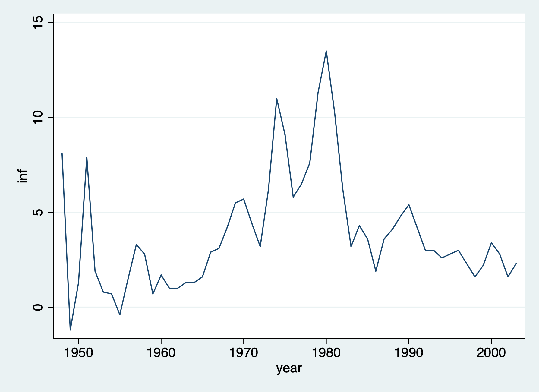
. use phillips.dta, clear
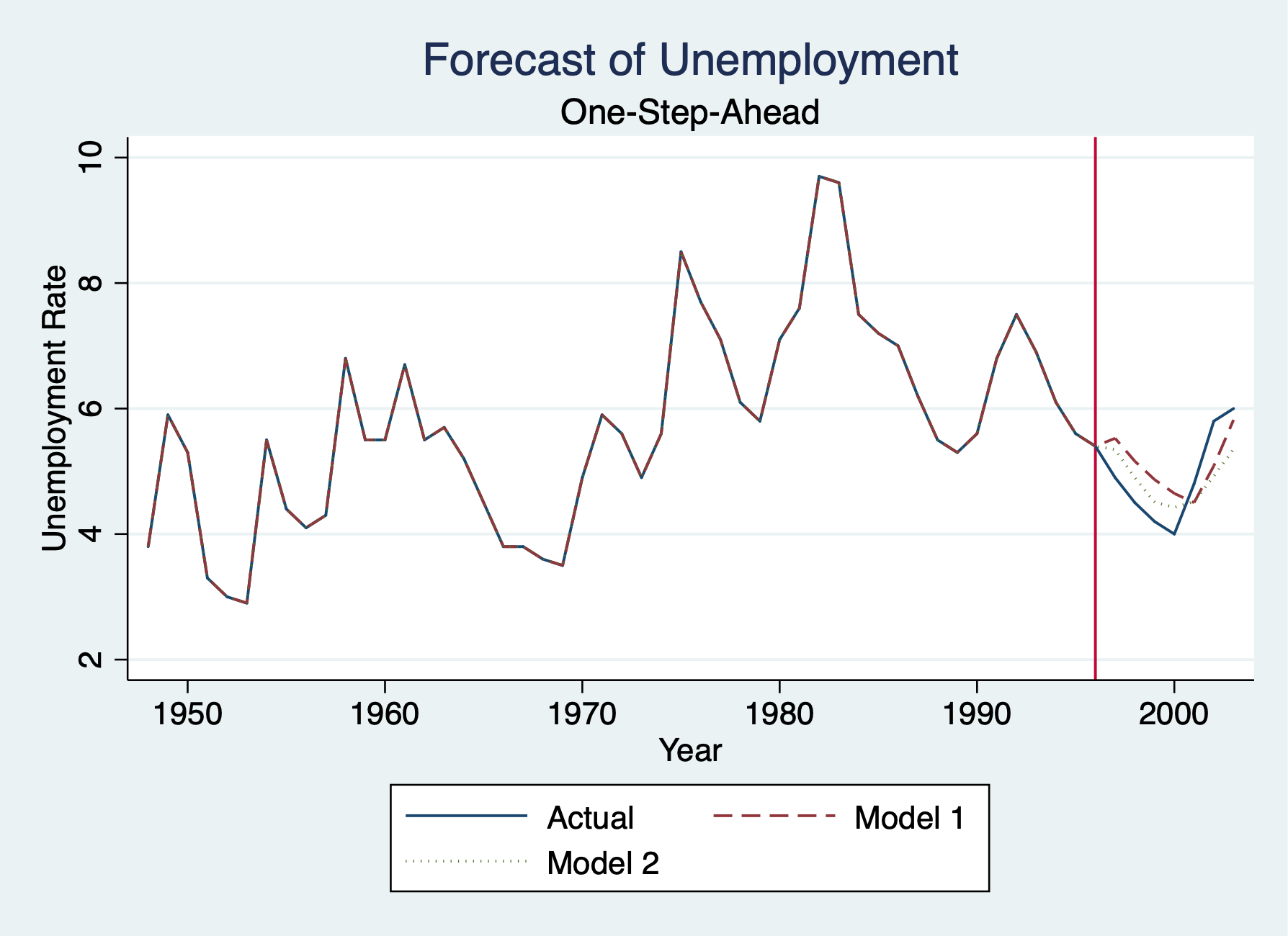
We’ll use our Phillip’s Curve data to forecast unemployment one-step into the future
Set Time Series
. tsset year
        time variable:  year, 1948 to 2003
                delta:  1 unit
tsline
. tsline inf

. graph export "/Users/Sam/Desktop/Econ 645/Stata/week_11_inflation.png", replace
(file /Users/Sam/Desktop/Econ 645/Stata/week_11_inflation.png written in PNG format)
First we need to Generate training and test samples, so we’ll use the time series sequence until 1996 as our training data, and we’ll use 1997 to 2003 as our testing data.
. gen test = 0

. replace test = 1 if year >= 1997
(7 real changes made)

. label define test1 0 "training sample" 1 "testing sample"

. label values test test1
We’ll use two models to forecast unemployment:
Compare models OLS AR(1)
. reg unem l.unem if test == 0

      Source │       SS           df       MS      Number of obs   =        48
─────────────┼──────────────────────────────────   F(1, 46)        =     57.13
       Model │  62.8162728         1  62.8162728   Prob > F        =    0.0000
    Residual │  50.5768515        46  1.09949677   R-squared       =    0.5540
─────────────┼──────────────────────────────────   Adj R-squared   =    0.5443
       Total │  113.393124        47  2.41261967   Root MSE        =    1.0486

─────────────┬────────────────────────────────────────────────────────────────
        unem │      Coef.   Std. Err.      t    P>|t|     [95% Conf. Interval]
─────────────┼────────────────────────────────────────────────────────────────
        unem │
         L1. │   .7323538   .0968906     7.56   0.000      .537323    .9273845
             │
       _cons │   1.571741   .5771181     2.72   0.009     .4100629     2.73342
─────────────┴────────────────────────────────────────────────────────────────
VAR - Add Lagged Inflation
. reg unem l.unem l.inf if test == 0

      Source │       SS           df       MS      Number of obs   =        48
─────────────┼──────────────────────────────────   F(2, 45)        =     50.22
       Model │  78.3083336         2  39.1541668   Prob > F        =    0.0000
    Residual │  35.0847907        45  .779662015   R-squared       =    0.6906
─────────────┼──────────────────────────────────   Adj R-squared   =    0.6768
       Total │  113.393124        47  2.41261967   Root MSE        =    .88298

─────────────┬────────────────────────────────────────────────────────────────
        unem │      Coef.   Std. Err.      t    P>|t|     [95% Conf. Interval]
─────────────┼────────────────────────────────────────────────────────────────
        unem │
         L1. │   .6470261   .0838056     7.72   0.000     .4782329    .8158192
             │
         inf │
         L1. │   .1835766   .0411828     4.46   0.000     .1006302    .2665231
             │
       _cons │   1.303797   .4896861     2.66   0.011     .3175188    2.290076
─────────────┴────────────────────────────────────────────────────────────────
One-step ahead we can use predict or forecast for AR(1)
. quietly reg unem l.unem if test == 0

. estimates store model1
We can get one-step ahead just using predict
. predict unem_est
(option xb assumed; fitted values)
(1 missing value generated)
Forecast - One-step-ahead forecast
. forecast create forecast1, replace
  (Forecast model forecast2 ended.)
  Forecast model forecast1 started.

. forecast estimates model1
  Added estimation results from regress.
  Forecast model forecast1 now contains 1 endogenous variable.
For a one-step ahead forecast, static is our key option otherwise it will not be a one-step ahead forecast.
. forecast solve, prefix(st_) begin(1997) end(2003) static

Computing static forecasts for model forecast1.
───────────────────────────────────────────────
Starting period:  1997
Ending period:    2003
Forecast prefix:  st_

1997:  .............
1998:  .............
1999:  ..............
2000:  ..............
2001:  ..............
2002:  .............
2003:  ............

Forecast 1 variable spanning 7 periods.
───────────────────────────────────────
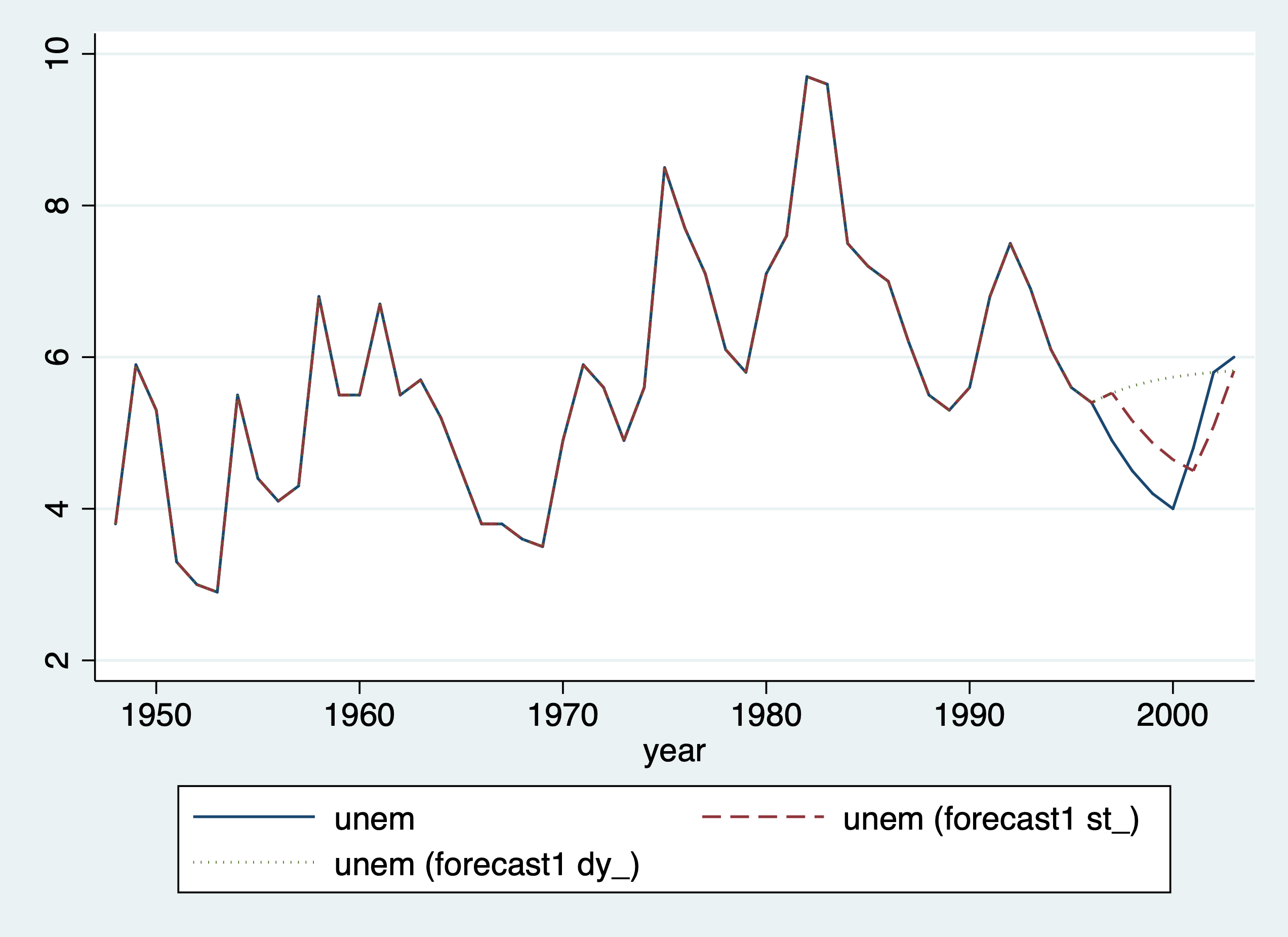
Dynamic model - We won’t use l.unem but l.dy_unem
. forecast solve, prefix(dy_) begin(1997) end(2003)

Computing dynamic forecasts for model forecast1.
────────────────────────────────────────────────
Starting period:  1997
Ending period:    2003
Forecast prefix:  dy_

1997:  .............
1998:  .............
1999:  ............
2000:  ............
2001:  ............
2002:  ............
2003:  ............

Forecast 1 variable spanning 7 periods.
───────────────────────────────────────
Graph Actual, One-Step-Ahead Model, and Dynamic Model
. twoway line unem year || line st_unem year, lpattern(dash) || line dy_unem year, lpattern(dot)

. graph export "/Users/Sam/Desktop/Econ 645/Stata/week_11_static_v_dynamic.png", replace
(file /Users/Sam/Desktop/Econ 645/Stata/week_11_static_v_dynamic.png written in PNG format)
Calculate RMSE for Model 1
. gen e = unem - st_unem

. gen e2 = e^2

. sum e2 if test==1

    Variable │        Obs        Mean    Std. Dev.       Min        Max
─────────────┼─────────────────────────────────────────────────────────
          e2 │          7    .3319141    .1891047   .0326187   .5083123

. scalar esum= `r(sum)'/`r(N)'

. scalar model1_RMSE= esum^.5

. display model1_RMSE
.57611988
Calculate MAE for Model 1
. gen e_abs = abs(e) if test ==1
(49 missing values generated)

. sum e_abs if test==1

    Variable │        Obs        Mean    Std. Dev.       Min        Max
─────────────┼─────────────────────────────────────────────────────────
       e_abs │          7     .542014    .2109284   .1806064   .7129602

. scalar model1_MAE=`r(mean)'

. display model1_MAE
.54201399
One-step ahead we can use predict or forecast for VAR Model (lagged employment and lagged inflation) Get 1997 estimates
. quietly reg unem l.unem l.inf if year < 1997
Our predict command will produce the same results as forecast solve, static
. predict p2
(option xb assumed; fitted values)
(1 missing value generated)

. estimates store model2
Forecast for Model 2
. forecast create forecast2, replace
  (Forecast model forecast1 ended.)
  Forecast model forecast2 started.

. forecast estimates model2
  Added estimation results from regress.
  Forecast model forecast2 now contains 1 endogenous variable.
One-Step-Ahead Forecast of Model 2
. forecast solve, prefix(st2_) begin(1997) end(2003) static

Computing static forecasts for model forecast2.
───────────────────────────────────────────────
Starting period:  1997
Ending period:    2003
Forecast prefix:  st2_

1997:  ............
1998:  ...........
1999:  ...........
2000:  .............
2001:  ..............
2002:  .............
2003:  ..............

Forecast 1 variable spanning 7 periods.
───────────────────────────────────────
Dynamic Forecast of Model 2
. forecast solve, prefix(dy2_) begin(1997) end(2003)

Computing dynamic forecasts for model forecast2.
────────────────────────────────────────────────
Starting period:  1997
Ending period:    2003
Forecast prefix:  dy2_

1997:  ............
1998:  .............
1999:  .............
2000:  ............
2001:  .............
2002:  ............
2003:  .............

Forecast 1 variable spanning 7 periods.
───────────────────────────────────────
Calculate RMSE for Model 2
. drop e e2 e_abs

. gen e = unem - st2_unem

. gen e2 = e^2

. sum e2 if test==1

    Variable │        Obs        Mean    Std. Dev.       Min        Max
─────────────┼─────────────────────────────────────────────────────────
          e2 │          7    .2722276    .2459784    .080621   .7681881

. scalar esum2 = `r(sum)'/`r(N)'

. scalar model2_RMSE=esum2^.5

. display model2_RMSE
.52175434
Calculate MAE for Model 2
. gen e_abs = abs(e)

. sum e_abs if test==1

    Variable │        Obs        Mean    Std. Dev.       Min        Max
─────────────┼─────────────────────────────────────────────────────────
       e_abs │          7    .4841946    .2099534   .2839384   .8764634

. scalar model2_MAE=`r(mean)'
Results
. display "Model 1: RMSE="model1_RMSE " and MAE="model1_MAE
Model 1: RMSE=.57611988 and MAE=.54201399

. display "Model 2: RMSE="model2_RMSE " and MAE="model1_MAE
Model 2: RMSE=.52175434 and MAE=.54201399

. display "Model 2 with lagged unemployment and lagged inflation has lower RMSE and MAE."
Model 2 with lagged unemployment and lagged inflation has lower RMSE and MAE.
Forecasting Line
. twoway line unem year || line st_unem year, lpattern(dash) || line st2_unem year, lpattern(dot) ///
> title("Forecast of Unemployment") xtitle("Year") subtitle("One-Step-Ahead") ytitle("Unemployment Rate") xline(199
> 6) ///
> legend(order(1 "Actual" 2 "Model 1" 3 "Model 2"))

. graph export "/Users/Sam/Desktop/Econ 645/Stata/week_11_forecast.png", replace
(file /Users/Sam/Desktop/Econ 645/Stata/week_11_forecast.png written in PNG format)