Samuel Rowe adapted from Wooldridge
Set Working Directory
. cd "/Users/Sam/Desktop/Econ 645/Data/Wooldridge"
/Users/Sam/Desktop/Econ 645/Data/Wooldridge
Topics:
. use phillips.dta, clear
*Set the Time Series
. tsset year, yearly
        time variable:  year, 1948 to 2003
                delta:  1 year
. reg inf unem if year < 1997

      Source │       SS           df       MS      Number of obs   =        49
─────────────┼──────────────────────────────────   F(1, 47)        =      2.62
       Model │  25.6369575         1  25.6369575   Prob > F        =    0.1125
    Residual │   460.61979        47  9.80042107   R-squared       =    0.0527
─────────────┼──────────────────────────────────   Adj R-squared   =    0.0326
       Total │  486.256748        48  10.1303489   Root MSE        =    3.1306

─────────────┬────────────────────────────────────────────────────────────────
         inf │      Coef.   Std. Err.      t    P>|t|     [95% Conf. Interval]
─────────────┼────────────────────────────────────────────────────────────────
        unem │   .4676257   .2891262     1.62   0.112    -.1140213    1.049273
       _cons │    1.42361   1.719015     0.83   0.412    -2.034602    4.881822
─────────────┴────────────────────────────────────────────────────────────────
Our result do not suggest a trade off between inflation and unemployment, and potentially suggest a positive relationship. This is likely a misspecified model and does not best describe the short-run trade-off between inflation and unemployment. We’ll look at an augmented Phillips curve that better describes the relationship.
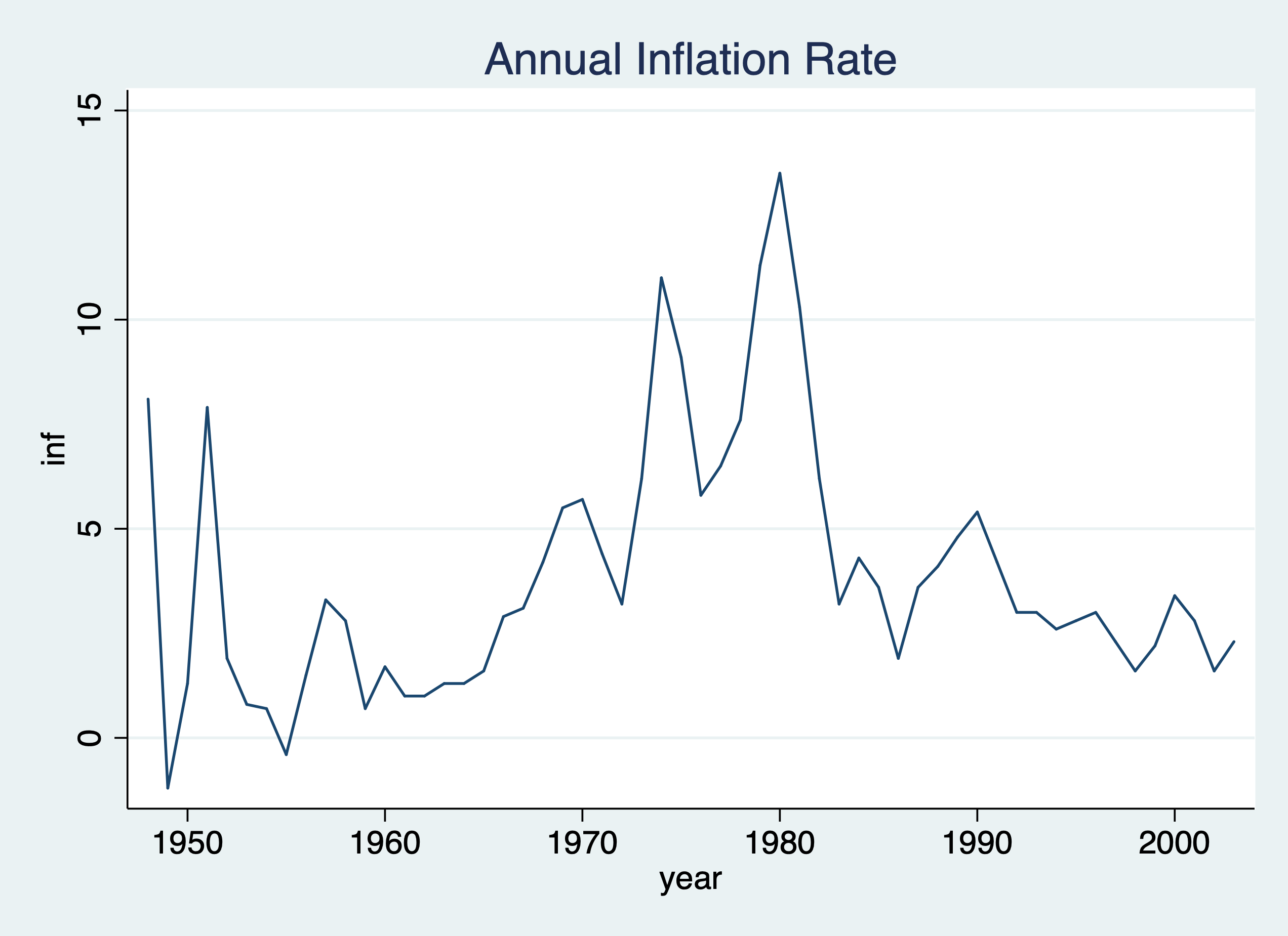
Let’s graph our time series
. twoway line inf year, title("Annual Inflation Rate")

. graph export "/Users/Sam/Desktop/Econ 645/Stata/week_10_inf_line.png", replace
(file /Users/Sam/Desktop/Econ 645/Stata/week_10_inf_line.png written in PNG format)
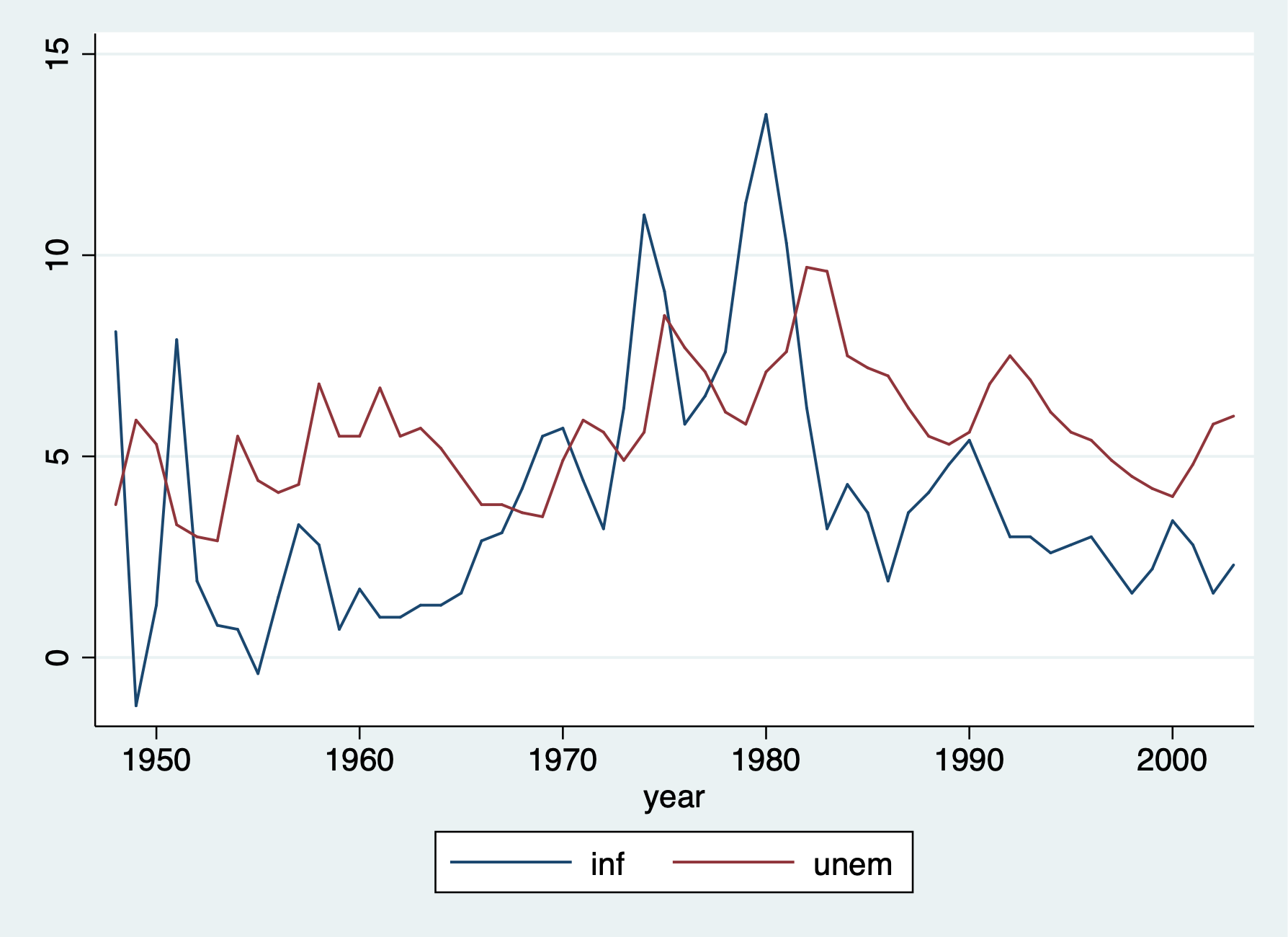
We can use tsline as well.
. tsline inf unem

. graph export "/Users/Sam/Desktop/Econ 645/Stata/week_10_ts_infemp.png", replace
(file /Users/Sam/Desktop/Econ 645/Stata/week_10_ts_infemp.png written in PNG format)
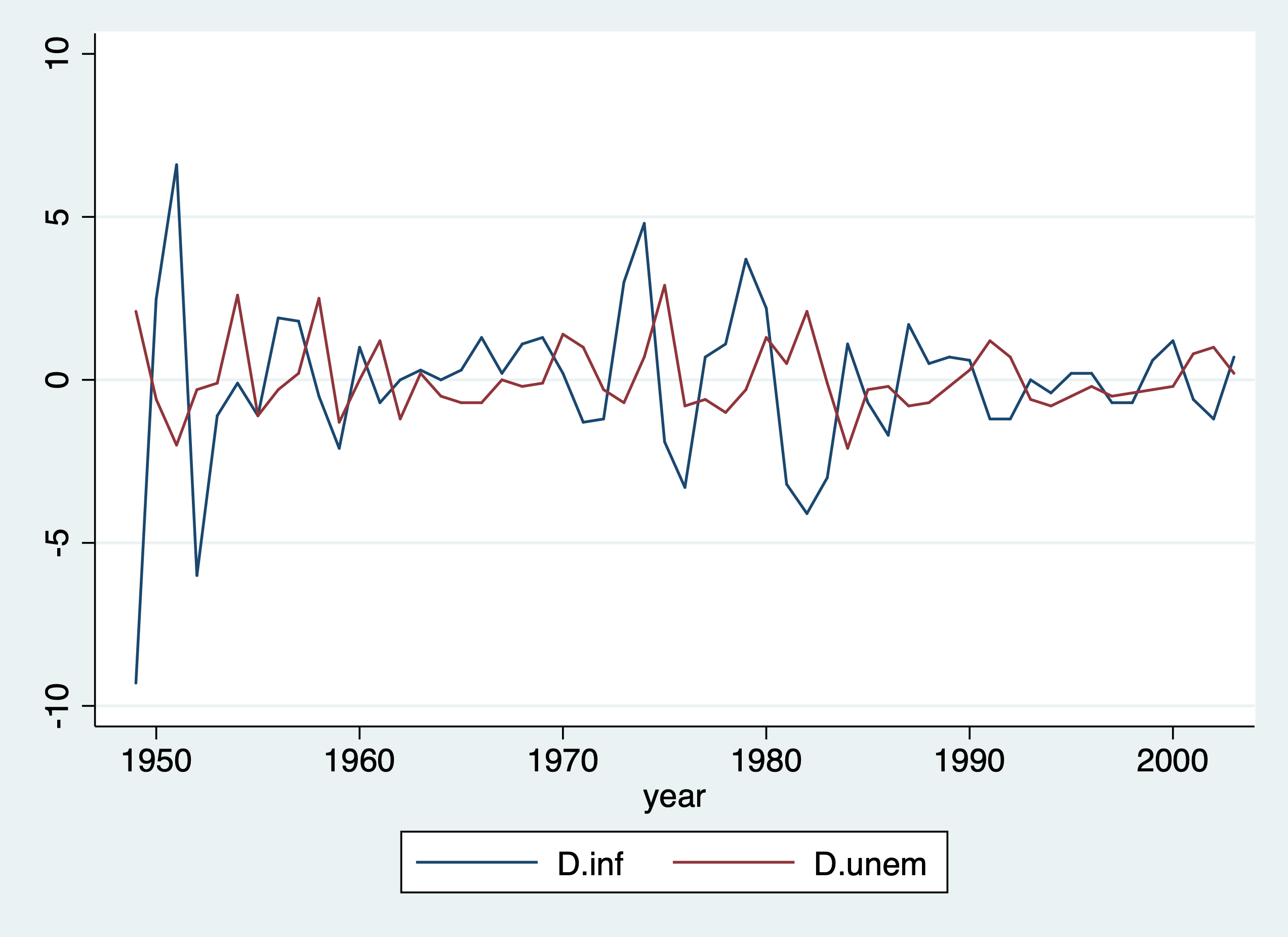
We can take the difference in the time series as well.
. tsline d.inf d.unem

. graph export "/Users/Sam/Desktop/Econ 645/Stata/week_10_ts_Dinfemp.png", replace
(file /Users/Sam/Desktop/Econ 645/Stata/week_10_ts_Dinfemp.png written in PNG format)
Caution: \[ D2. \neq S2. \] It is not recommended to use d. beyond the first difference. Use the S12. operator If you are interested in \[ x_{t}-x_{t-12} = \Delta x \] D2 gives the difference in differences (not the research design. Such that D2.
operator calculates: \[ D2 = x_{t} - x_{t-1} - (x_{t-1}-x_{t-2}) \] \[ S2 = x_{t} - x_{t-2} \]
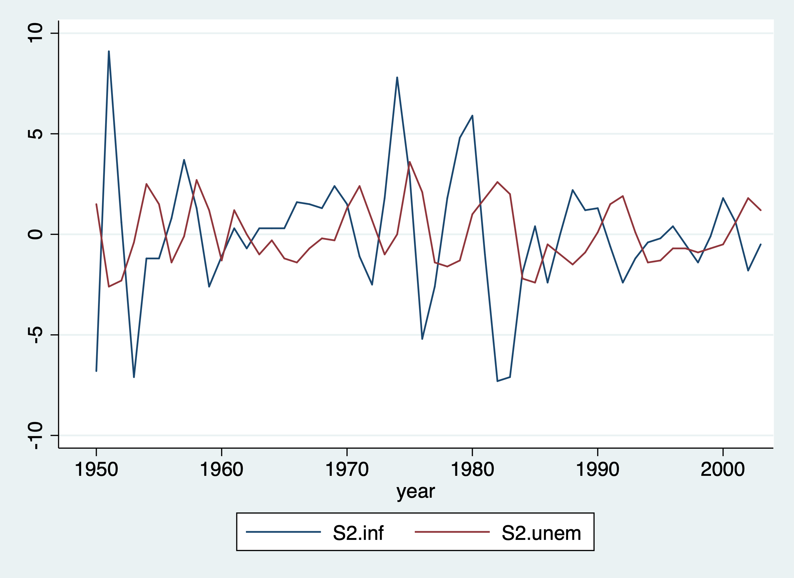
We can take the 12-month difference in the time series as well.
. tsline s2.inf s2.unem

. graph export "/Users/Sam/Desktop/Econ 645/Stata/week_10_ts_D12infemp.png", replace
(file /Users/Sam/Desktop/Econ 645/Stata/week_10_ts_D12infemp.png written in PNG format)
. use intdef.dta, clearLooking inflation and deficits on interest rates, our model is: \[ i3_t = \beta_0 + \beta_1 inflation_t + \beta_2 deficitpct_t + u_t \] Where
Set the Time Series
. tsset year
        time variable:  year, 1948 to 2003
                delta:  1 unit
. reg i3 inf def if year < 2004

      Source │       SS           df       MS      Number of obs   =        56
─────────────┼──────────────────────────────────   F(2, 53)        =     40.09
       Model │  272.420338         2  136.210169   Prob > F        =    0.0000
    Residual │  180.054275        53  3.39725047   R-squared       =    0.6021
─────────────┼──────────────────────────────────   Adj R-squared   =    0.5871
       Total │  452.474612        55  8.22681113   Root MSE        =    1.8432

─────────────┬────────────────────────────────────────────────────────────────
          i3 │      Coef.   Std. Err.      t    P>|t|     [95% Conf. Interval]
─────────────┼────────────────────────────────────────────────────────────────
         inf │   .6058659   .0821348     7.38   0.000     .4411243    .7706074
         def │   .5130579   .1183841     4.33   0.000     .2756095    .7505062
       _cons │   1.733266    .431967     4.01   0.000     .8668497    2.599682
─────────────┴────────────────────────────────────────────────────────────────
This static model better explain interest rates based on basic macroeconomics. Both contemporaneous variables explain current interest rates. A 1 percentage point increase in the inflation rate leads to a 0.6 percentage point increase in the nominal interest rate. A 1 percentage point increase in the deficits as a percentage of GDP leads to a 0.5 percentage point increase in nominal interest rates.
. use prminwge, clearWe’ll look at the association between employment and minimum wage in Puerto Rico. Our model will be: \[ lprepop_t = \beta_0 + \beta_1 lmincov_t + \beta_2 lusgnp + u_t \] Where
Set Time Series
. tsset year
        time variable:  year, 1950 to 1987
                delta:  1 unit
. reg lprepop lmincov lusgnp if year < 1988

      Source │       SS           df       MS      Number of obs   =        38
─────────────┼──────────────────────────────────   F(2, 35)        =     34.04
       Model │  .211258366         2  .105629183   Prob > F        =    0.0000
    Residual │  .108600151        35  .003102861   R-squared       =    0.6605
─────────────┼──────────────────────────────────   Adj R-squared   =    0.6411
       Total │  .319858518        37  .008644825   Root MSE        =     .0557

─────────────┬────────────────────────────────────────────────────────────────
     lprepop │      Coef.   Std. Err.      t    P>|t|     [95% Conf. Interval]
─────────────┼────────────────────────────────────────────────────────────────
     lmincov │  -.1544442   .0649015    -2.38   0.023    -.2862011   -.0226872
      lusgnp │  -.0121888   .0885134    -0.14   0.891    -.1918806     .167503
       _cons │  -1.054423   .7654065    -1.38   0.177     -2.60828    .4994351
─────────────┴────────────────────────────────────────────────────────────────
Our results show that there is a tradeoff between the employment ratio and the importance of minimum wage. A one percent increase in importance of minimum wage the employment-population ratio declines .154 percent.
The barium industry in the U.S. complained to the International Trade Commission that China was dumping (or selling imports at lower prices to undercut domestic producers). First, are imports unusually high before the complaint? Second, do imports change after the dumping complaint?
. use barium.dta, clear
Set Time Series Monthly
. tsset t, monthly
        time variable:  t, 1960m2 to 1970m12
                delta:  1 month
Our model is the \[ lchnimp_t = \beta_0 + \beta_1 lchempi_t + \beta_2 lgas_t + \beta_3 lrtwex_t +\beta_4 befile6_t + \beta_5 affile6_t + \beta_6 afdec6 + u_t \]
. reg lchnimp lchempi lgas lrtwex befile6 affile6 afdec6

      Source │       SS           df       MS      Number of obs   =       131
─────────────┼──────────────────────────────────   F(6, 124)       =      9.06
       Model │  19.4051607         6  3.23419346   Prob > F        =    0.0000
    Residual │  44.2470875       124  .356831351   R-squared       =    0.3049
─────────────┼──────────────────────────────────   Adj R-squared   =    0.2712
       Total │  63.6522483       130  .489632679   Root MSE        =    .59735

─────────────┬────────────────────────────────────────────────────────────────
     lchnimp │      Coef.   Std. Err.      t    P>|t|     [95% Conf. Interval]
─────────────┼────────────────────────────────────────────────────────────────
     lchempi │   3.117193   .4792021     6.50   0.000     2.168718    4.065668
        lgas │   .1963504   .9066172     0.22   0.829    -1.598099      1.9908
      lrtwex │   .9830183   .4001537     2.46   0.015     .1910022    1.775034
     befile6 │   .0595739   .2609699     0.23   0.820    -.4569585    .5761064
     affile6 │  -.0324064   .2642973    -0.12   0.903    -.5555249     .490712
      afdec6 │   -.565245   .2858352    -1.98   0.050    -1.130993    .0005028
       _cons │    -17.803   21.04537    -0.85   0.399    -59.45769    23.85169
─────────────┴────────────────────────────────────────────────────────────────
We see that imports are not higher 6 months before a complaint, and imports are not lower 6 months after a complaint. However, imports are lower 6 months after a positive decision in a complaint by the ITC. The impact is fairly large and imports of barium chloride fall about 43.2% after a positive decision.
Also notice that rtwex is positive, and we would expect that a stronger dollar increase demand for imports, which is about uni-elastic.
. display (exp(-.565)-1)*100
-43.163985
Lesson: using lags in the explanatory variables Personal Exemption on Fertility Rates
. use fertil3.dta, clear
Our interest the general fertility rate, which is the number of children born to every 1,000 women of childbearing age. PE is the average real dollar value of the personal tax exemption and two binary variables for World War II and the introduction of the birth control pill in 1963.
Our contemporenous model is: \[ gfr_t=\beta_0 + \beta_1 pe_t + \beta_2 ww2_t + \beta_3 pill_t + u_t \]
WhereSet Time Series
. tsset year, yearly
        time variable:  year, 1913 to 1984
                delta:  1 year
. reg gfr pe i.ww2 i.pill if year < 1985

      Source │       SS           df       MS      Number of obs   =        72
─────────────┼──────────────────────────────────   F(3, 68)        =     20.38
       Model │  13183.6215         3  4394.54049   Prob > F        =    0.0000
    Residual │  14664.2739        68  215.651087   R-squared       =    0.4734
─────────────┼──────────────────────────────────   Adj R-squared   =    0.4502
       Total │  27847.8954        71  392.223879   Root MSE        =    14.685

─────────────┬────────────────────────────────────────────────────────────────
         gfr │      Coef.   Std. Err.      t    P>|t|     [95% Conf. Interval]
─────────────┼────────────────────────────────────────────────────────────────
          pe │     .08254   .0296462     2.78   0.007     .0233819    .1416981
       1.ww2 │   -24.2384   7.458253    -3.25   0.002    -39.12111   -9.355684
      1.pill │  -31.59403   4.081068    -7.74   0.000    -39.73768   -23.45039
       _cons │   98.68176   3.208129    30.76   0.000     92.28003    105.0835
─────────────┴────────────────────────────────────────────────────────────────
World War II reduced the fertility rate by 24.24 births per 1,000 women of child bearing age, while the introduction of the birth control pill reduced the number of birth by 31.59 births per 1,000 women of childbearing age. The personal tax exemption. A one dollar increase in the average real value of the personal tax exemption increases 0.083 births per 1,000 women of child bearing age or a 12 dollar increase in the average real personal tax exemption increases 1 child per 1,000 women of child bearing ago
Next lets add lags in the average real value of the personal tax exemption. Our Finite Distributed Lag model is: \[ gfr_t=\beta_0 + \beta_1 pe_t + \beta_2 pe_{t-1} + \beta_3 pe_{t-2} + \beta_4 ww2_t + \beta_5 pill_t + u_t \]
. reg gfr pe pe_1 pe_2 i.ww2 i.pill if year < 1985

      Source │       SS           df       MS      Number of obs   =        70
─────────────┼──────────────────────────────────   F(5, 64)        =     12.73
       Model │  12959.7886         5  2591.95772   Prob > F        =    0.0000
    Residual │  13032.6443        64  203.635067   R-squared       =    0.4986
─────────────┼──────────────────────────────────   Adj R-squared   =    0.4594
       Total │  25992.4329        69  376.701926   Root MSE        =     14.27

─────────────┬────────────────────────────────────────────────────────────────
         gfr │      Coef.   Std. Err.      t    P>|t|     [95% Conf. Interval]
─────────────┼────────────────────────────────────────────────────────────────
          pe │   .0726718   .1255331     0.58   0.565    -.1781094     .323453
        pe_1 │  -.0057796   .1556629    -0.04   0.970     -.316752    .3051929
        pe_2 │   .0338268   .1262574     0.27   0.790    -.2184013     .286055
       1.ww2 │   -22.1265   10.73197    -2.06   0.043    -43.56608   -.6869196
      1.pill │  -31.30499   3.981559    -7.86   0.000    -39.25907   -23.35091
       _cons │    95.8705   3.281957    29.21   0.000     89.31403     102.427
─────────────┴────────────────────────────────────────────────────────────────
Our personal exemption variables are no longer statistically significiant, but let’s test the joint significance. We might have multicollinearity that bias our standard errors for our PE variables.
. test pe pe_1 pe_2

 ( 1)  pe = 0
 ( 2)  pe_1 = 0
 ( 3)  pe_2 = 0

       F(  3,    64) =    3.97
            Prob > F =    0.0117

. test pe_1 pe_2

 ( 1)  pe_1 = 0
 ( 2)  pe_2 = 0

       F(  2,    64) =    0.05
            Prob > F =    0.9480
Our PE variables are jointly significant, but our lags are jointly insignificiant so we’ll use our static model.
For the estimated LRP: .073-.0058+0.034~.101, but we lack a standard error. We’ll need to estimate the standard error. Let \[ \theta_0=\delta_0+\delta_1+\delta_2 \] denote the LRP and write \[ \delta_0 \] in terms of \[ \theta_0 \, , \delta_1 \, and \, \delta_2 \, where \, \delta_0 = \theta_0 - \delta_1 - \delta_2 \] Next substitute for \[ \delta_0 \] \[ gfr_t = \alpha_0 + \delta_0 pe_t + \delta_1 pe_{t-1} + \delta_2 pe_{t-2} + ... \] to get \[ gfr_t = \alpha_0 + (\theta_0 - \delta_1 - \delta_2)pe_t + \delta_1 pe_{t-1} + \delta_2 pe_{t-2} + ... \] \[ gfr_t = \alpha_0 + \theta_0 pe_t + \delta_1 (pe_{t-1} - pe_t) + \delta_2 (pe_{t-2} - pe_t) + \]
We can estimate \[ \hat{\theta}_{0} \] and its standard error. We can regress gfr_t onto pe_t, (pe_(t-1) - pe_t), and (pe_t-2 - pe_t), ww2, and pill
. gen pe_1_1 = pe_1 - pe
(1 missing value generated)

. gen pe_2_1 = pe_2 - pe
(2 missing values generated)
. reg gfr pe pe_1_1 pe_2_1 i.ww2 i.pill

      Source │       SS           df       MS      Number of obs   =        70
─────────────┼──────────────────────────────────   F(5, 64)        =     12.73
       Model │  12959.7886         5  2591.95772   Prob > F        =    0.0000
    Residual │  13032.6443        64  203.635067   R-squared       =    0.4986
─────────────┼──────────────────────────────────   Adj R-squared   =    0.4594
       Total │  25992.4329        69  376.701926   Root MSE        =     14.27

─────────────┬────────────────────────────────────────────────────────────────
         gfr │      Coef.   Std. Err.      t    P>|t|     [95% Conf. Interval]
─────────────┼────────────────────────────────────────────────────────────────
          pe │   .1007191   .0298027     3.38   0.001     .0411814    .1602568
      pe_1_1 │  -.0057796   .1556629    -0.04   0.970     -.316752    .3051929
      pe_2_1 │   .0338268   .1262574     0.27   0.790    -.2184013     .286055
       1.ww2 │   -22.1265   10.73197    -2.06   0.043    -43.56608   -.6869196
      1.pill │  -31.30499   3.981559    -7.86   0.000    -39.25907   -23.35091
       _cons │    95.8705   3.281957    29.21   0.000     89.31403     102.427
─────────────┴────────────────────────────────────────────────────────────────
Our theta-hat is about .101 and significant, so our LRP has an effect on general fertility rates.
. use hseinv.dta, clear
We look at annual housing investement and a housing price index from 1947 to 1988.
Set Time Series
. tsset year, yearly
        time variable:  year, 1947 to 1988
                delta:  1 year
Our model is the natural log of invpc or real per capita housing investment ($1,000) and price be the housing price index where 1982 = 1 (or 100). We’ll assume constant elasticity with our log-log model.
\[ linvpc = \beta_0 + \beta_1 lprice_t + u_t \]
. reg linvpc lprice

      Source │       SS           df       MS      Number of obs   =        42
─────────────┼──────────────────────────────────   F(1, 40)        =     10.53
       Model │  .254364468         1  .254364468   Prob > F        =    0.0024
    Residual │  .966255566        40  .024156389   R-squared       =    0.2084
─────────────┼──────────────────────────────────   Adj R-squared   =    0.1886
       Total │  1.22062003        41   .02977122   Root MSE        =    .15542

─────────────┬────────────────────────────────────────────────────────────────
      linvpc │      Coef.   Std. Err.      t    P>|t|     [95% Conf. Interval]
─────────────┼────────────────────────────────────────────────────────────────
      lprice │   1.240943   .3824192     3.24   0.002     .4680452    2.013841
       _cons │  -.5502345   .0430266   -12.79   0.000    -.6371945   -.4632746
─────────────┴────────────────────────────────────────────────────────────────
Our output shows that a 1 percent increase in the pricing index increases the investment per capita by 1.24 percent (or elastic response). Note: both investment and price have upward trends that we need to account for.
\[ invpc = \beta_0 + \beta_1 lprice_t + \beta_2 t + u_t \]
. reg linvpc lprice t

      Source │       SS           df       MS      Number of obs   =        42
─────────────┼──────────────────────────────────   F(2, 39)        =     10.08
       Model │  .415945108         2  .207972554   Prob > F        =    0.0003
    Residual │  .804674927        39   .02063269   R-squared       =    0.3408
─────────────┼──────────────────────────────────   Adj R-squared   =    0.3070
       Total │  1.22062003        41   .02977122   Root MSE        =    .14364

─────────────┬────────────────────────────────────────────────────────────────
      linvpc │      Coef.   Std. Err.      t    P>|t|     [95% Conf. Interval]
─────────────┼────────────────────────────────────────────────────────────────
      lprice │  -.3809612   .6788352    -0.56   0.578    -1.754035    .9921125
           t │   .0098287   .0035122     2.80   0.008     .0027246    .0169328
       _cons │  -.9130595   .1356133    -6.73   0.000    -1.187363   -.6387557
─────────────┴────────────────────────────────────────────────────────────────
After accounting for the upward linear trend for both investment per capita and the housing price index, an increase in price is coefficient is now negative, but it is not statistically significant. We probably have serial correlation which will bias our standard errors.
. predict u, resid

. reg u l.u, noconst

      Source │       SS           df       MS      Number of obs   =        41
─────────────┼──────────────────────────────────   F(1, 40)        =     11.10
       Model │  .170666637         1  .170666637   Prob > F        =    0.0019
    Residual │  .614779847        40  .015369496   R-squared       =    0.2173
─────────────┼──────────────────────────────────   Adj R-squared   =    0.1977
       Total │  .785446484        41  .019157231   Root MSE        =    .12397

─────────────┬────────────────────────────────────────────────────────────────
           u │      Coef.   Std. Err.      t    P>|t|     [95% Conf. Interval]
─────────────┼────────────────────────────────────────────────────────────────
           u │
         L1. │   .4632581   .1390204     3.33   0.002     .1822874    .7442288
─────────────┴────────────────────────────────────────────────────────────────

. drop u
. use fertil3.dta, clear
We’ll look at fertility again, but we’ll account for a quadratic time trend. First, we’ll estimate a linear time trend, and then we’ll try a quadratic time trend.
Set Time Series
. tsset year, yearly
        time variable:  year, 1913 to 1984
                delta:  1 year
Linear Trend
. reg gfr pe i.ww2 i.pill t if year < 1985

      Source │       SS           df       MS      Number of obs   =        72
─────────────┼──────────────────────────────────   F(4, 67)        =     32.84
       Model │  18441.2357         4  4610.30894   Prob > F        =    0.0000
    Residual │  9406.65967        67  140.397905   R-squared       =    0.6622
─────────────┼──────────────────────────────────   Adj R-squared   =    0.6420
       Total │  27847.8954        71  392.223879   Root MSE        =    11.849

─────────────┬────────────────────────────────────────────────────────────────
         gfr │      Coef.   Std. Err.      t    P>|t|     [95% Conf. Interval]
─────────────┼────────────────────────────────────────────────────────────────
          pe │   .2788778   .0400199     6.97   0.000     .1989978    .3587578
       1.ww2 │  -35.59228   6.297377    -5.65   0.000     -48.1619   -23.02266
      1.pill │   .9974479    6.26163     0.16   0.874    -11.50082    13.49571
           t │  -1.149872   .1879038    -6.12   0.000    -1.524929   -.7748145
       _cons │   111.7694   3.357765    33.29   0.000     105.0673    118.4716
─────────────┴────────────────────────────────────────────────────────────────
Quadratic Trend Fertility is declining but at a decreasing negatively rate (eventually a positive t^2 takes over t)
. reg gfr pe i.ww2 i.pill c.t##c.t if year < 1985

      Source │       SS           df       MS      Number of obs   =        72
─────────────┼──────────────────────────────────   F(5, 66)        =     35.09
       Model │  20236.3981         5  4047.27961   Prob > F        =    0.0000
    Residual │  7611.49734        66  115.325717   R-squared       =    0.7267
─────────────┼──────────────────────────────────   Adj R-squared   =    0.7060
       Total │  27847.8954        71  392.223879   Root MSE        =    10.739

─────────────┬────────────────────────────────────────────────────────────────
         gfr │      Coef.   Std. Err.      t    P>|t|     [95% Conf. Interval]
─────────────┼────────────────────────────────────────────────────────────────
          pe │   .3478126   .0402599     8.64   0.000     .2674311     .428194
       1.ww2 │  -35.88028   5.707921    -6.29   0.000    -47.27651   -24.48404
      1.pill │  -10.11972   6.336094    -1.60   0.115    -22.77014    2.530696
           t │  -2.531426   .3893863    -6.50   0.000    -3.308861   -1.753991
             │
     c.t#c.t │   .0196126    .004971     3.95   0.000     .0096876    .0295377
             │
       _cons │   124.0919   4.360738    28.46   0.000     115.3854    132.7984
─────────────┴────────────────────────────────────────────────────────────────
The fertility rate exhibits upward and downward trends between 1913 and 1984. Interestingly, pe remains fairly robust after adding time trends. The linear time trend shows that general fertility rates are falling by 1.15 childs per 1,000 women of childbearing age for each additional year. However, the quadratic shows that the trend is negative but decreasing rate and will eventually become positive.
The last linear trend is for employment-population ratio and the importance of minimum wage coverage. We’ll add a time trend along with mincov and usgnp.
. use prminwge, clear
Set the Time Series
. tsset year, yearly
        time variable:  year, 1950 to 1987
                delta:  1 year
Add linear trend
. reg lprepop lmincov lusgnp t

      Source │       SS           df       MS      Number of obs   =        38
─────────────┼──────────────────────────────────   F(3, 34)        =     62.78
       Model │  .270948453         3  .090316151   Prob > F        =    0.0000
    Residual │  .048910064        34  .001438531   R-squared       =    0.8471
─────────────┼──────────────────────────────────   Adj R-squared   =    0.8336
       Total │  .319858518        37  .008644825   Root MSE        =    .03793

─────────────┬────────────────────────────────────────────────────────────────
     lprepop │      Coef.   Std. Err.      t    P>|t|     [95% Conf. Interval]
─────────────┼────────────────────────────────────────────────────────────────
     lmincov │  -.1686949   .0442463    -3.81   0.001    -.2586142   -.0787757
      lusgnp │   1.057351   .1766369     5.99   0.000     .6983813     1.41632
           t │  -.0323542   .0050227    -6.44   0.000    -.0425616   -.0221468
       _cons │  -8.696298   1.295764    -6.71   0.000    -11.32961   -6.062988
─────────────┴────────────────────────────────────────────────────────────────
The employment-population ratio does not have much of a downward or upward trend, but usgnp does. Тhe linear trend of usgnp is about 3% per year, so an estimate of 1.06 in our model mean that when usgnp increases by 1% above its long-term trend, employment-population ratio increases by about 1.06%
We’ll add monthly variables to account for the fact that imports are not seasonlly adjusted.
. use barium.dta, clear
Set Time Series Monthly
. tsset t, monthly
        time variable:  t, 1960m2 to 1970m12
                delta:  1 month
. reg lchnimp lchempi lgas lrtwex befile6 affile6 afdec6 feb mar apr may ///
>     jun jul aug sep oct nov dec

      Source │       SS           df       MS      Number of obs   =       131
─────────────┼──────────────────────────────────   F(17, 113)      =      3.71
       Model │  22.8083523        17  1.34166778   Prob > F        =    0.0000
    Residual │   40.843896       113  .361450407   R-squared       =    0.3583
─────────────┼──────────────────────────────────   Adj R-squared   =    0.2618
       Total │  63.6522483       130  .489632679   Root MSE        =    .60121

─────────────┬────────────────────────────────────────────────────────────────
     lchnimp │      Coef.   Std. Err.      t    P>|t|     [95% Conf. Interval]
─────────────┼────────────────────────────────────────────────────────────────
     lchempi │    3.26506   .4929302     6.62   0.000     2.288476    4.241644
        lgas │  -1.278121   1.389008    -0.92   0.359    -4.029997    1.473755
      lrtwex │   .6630496   .4713038     1.41   0.162    -.2706882    1.596787
     befile6 │   .1397024   .2668075     0.52   0.602    -.3888914    .6682962
     affile6 │   .0126317   .2786866     0.05   0.964    -.5394967    .5647601
      afdec6 │  -.5213006     .30195    -1.73   0.087    -1.119518    .0769168
         feb │  -.4177089   .3044445    -1.37   0.173    -1.020868    .1854505
         mar │   .0590528   .2647308     0.22   0.824    -.4654266    .5835322
         apr │  -.4514825   .2683865    -1.68   0.095    -.9832046    .0802396
         may │   .0333085   .2692425     0.12   0.902    -.5001093    .5667264
         jun │  -.2063321   .2692515    -0.77   0.445    -.7397679    .3271038
         jul │   .0038354   .2787665     0.01   0.989    -.5484513    .5561222
         aug │  -.1570652   .2779928    -0.56   0.573    -.7078191    .3936887
         sep │  -.1341606   .2676556    -0.50   0.617    -.6644348    .3961135
         oct │   .0516921   .2668512     0.19   0.847    -.4769883    .5803725
         nov │    -.24626   .2628272    -0.94   0.351     -.766968     .274448
         dec │   .1328368   .2714234     0.49   0.626    -.4049019    .6705755
       _cons │   16.77877   32.42865     0.52   0.606    -47.46824    81.02577
─────────────┴────────────────────────────────────────────────────────────────
We compare all months to January as the base period, but let’s test their joint significance.
. test feb mar apr may jun jul aug sep oct nov dec

 ( 1)  feb = 0
 ( 2)  mar = 0
 ( 3)  apr = 0
 ( 4)  may = 0
 ( 5)  jun = 0
 ( 6)  jul = 0
 ( 7)  aug = 0
 ( 8)  sep = 0
 ( 9)  oct = 0
 (10)  nov = 0
 (11)  dec = 0

       F( 11,   113) =    0.86
            Prob > F =    0.5852
We find that they are jointly insignificant and seasonality does not seem to be an issue with barium chloride imports.
We’ll test the a version of the efficient market hypothesis (EMH) by looking at weekly stock return from 1976 to 1989.
. use nyse, clear
*Set Time Series
. tsset t, weekly
        time variable:  t, 1960w2 to 1973w16
                delta:  1 week
Our dependent variable is the weekly percentage return on the New York Stock Exchange. A strict form of the EMH states that information observable to the market prior to week t should not help to predict the return during week t. \[ E(y_t|y_{t-1},y_{t-2},...)=E(y_t) \]
We will test EMH by specifying an AR(1) model and our hypothesis states that beta for y_(t-1) will be equal to 0. We’ll assume that stock returns are serially uncorrelated, so we can safetly assume that they are weakly dependent.
\[ return_t = \beta_0 + \rho return_{t-1} + e_t \]
. reg return l.return

      Source │       SS           df       MS      Number of obs   =       689
─────────────┼──────────────────────────────────   F(1, 687)       =      2.40
       Model │  10.6866231         1  10.6866231   Prob > F        =    0.1218
    Residual │  3059.73817       687  4.45376735   R-squared       =    0.0035
─────────────┼──────────────────────────────────   Adj R-squared   =    0.0020
       Total │  3070.42479       688  4.46282673   Root MSE        =    2.1104

─────────────┬────────────────────────────────────────────────────────────────
      return │      Coef.   Std. Err.      t    P>|t|     [95% Conf. Interval]
─────────────┼────────────────────────────────────────────────────────────────
      return │
         L1. │   .0588984   .0380231     1.55   0.122    -.0157569    .1335538
             │
       _cons │    .179634   .0807419     2.22   0.026     .0211034    .3381646
─────────────┴────────────────────────────────────────────────────────────────
Or
. reg return return_1

      Source │       SS           df       MS      Number of obs   =       689
─────────────┼──────────────────────────────────   F(1, 687)       =      2.40
       Model │  10.6866231         1  10.6866231   Prob > F        =    0.1218
    Residual │  3059.73817       687  4.45376735   R-squared       =    0.0035
─────────────┼──────────────────────────────────   Adj R-squared   =    0.0020
       Total │  3070.42479       688  4.46282673   Root MSE        =    2.1104

─────────────┬────────────────────────────────────────────────────────────────
      return │      Coef.   Std. Err.      t    P>|t|     [95% Conf. Interval]
─────────────┼────────────────────────────────────────────────────────────────
    return_1 │   .0588984   .0380231     1.55   0.122    -.0157569    .1335538
       _cons │    .179634   .0807419     2.22   0.026     .0211034    .3381646
─────────────┴────────────────────────────────────────────────────────────────

. predict u, resid
(2 missing values generated)

. reg u l.u, noconst

      Source │       SS           df       MS      Number of obs   =       688
─────────────┼──────────────────────────────────   F(1, 687)       =      0.00
       Model │   .00603936         1   .00603936   Prob > F        =    0.9706
    Residual │  3059.08227       687  4.45281262   R-squared       =    0.0000
─────────────┼──────────────────────────────────   Adj R-squared   =   -0.0015
       Total │  3059.08831       688  4.44634929   Root MSE        =    2.1102

─────────────┬────────────────────────────────────────────────────────────────
           u │      Coef.   Std. Err.      t    P>|t|     [95% Conf. Interval]
─────────────┼────────────────────────────────────────────────────────────────
           u │
         L1. │    .001405   .0381496     0.04   0.971    -.0734987    .0763087
─────────────┴────────────────────────────────────────────────────────────────

. drop u
We cannot reject the null hypothesis under our model, but we do have some evidence of positive serial correlation.
We’ll revisit the Phillips curve
. use phillips.dta, clear
Set Time Series
. tsset year
        time variable:  year, 1948 to 2003
                delta:  1 unit
A linear version of the expections augmented Phillips curve can be written as \[ inf_t - inf^e_t=\beta_1(unemp_t-\mu_0) + e_t \]
Where mu_0 is the natural rate of unemployment and inf^e is the expected rate of inflation formed in year t-1. The difference between actual unemployment and the natural rate is called cyclical unemployment, while the difference between inflation and expected inflation is called unanticipated inflation Our e_t is called our supply shock. If there is a trade-off between inflation and unemployment our beta-hat_1 will be negative.
An assumption is made about inflationary expectations and unders adaptive expectations, the expected value of current inflation depends on recently observed inflation. The expected inflation will be assumed to be equal to last years inflation \[ inf_t - inf_{t-1}=\beta_0 + \beta_1 unemp_t + e_t \] \[ \Delta inf_t =\beta_0 + \beta_1 unemp_t + e_t \]
Where \[ \Delta inf_t=inf_t - inf_{t-1} \] \[ \beta_0 = -\beta_1 \mu_0 \] Since beta_1 is expected to be negative and beta_0 is expected to be positive.
Therefore, under adaptive expectations, the augmented Phillips curve relates the change in inflation to the level of unemployment and a supply shock e_t. We’ll assume assumptions TSC.1-TSC.5 hold.
First Difference in the dependent variable or adaptive expectations of inflation
. reg cinf unem if year < 1997

      Source │       SS           df       MS      Number of obs   =        48
─────────────┼──────────────────────────────────   F(1, 46)        =      5.56
       Model │  33.3830007         1  33.3830007   Prob > F        =    0.0227
    Residual │  276.305134        46  6.00663335   R-squared       =    0.1078
─────────────┼──────────────────────────────────   Adj R-squared   =    0.0884
       Total │  309.688135        47  6.58910925   Root MSE        =    2.4508

─────────────┬────────────────────────────────────────────────────────────────
        cinf │      Coef.   Std. Err.      t    P>|t|     [95% Conf. Interval]
─────────────┼────────────────────────────────────────────────────────────────
        unem │  -.5425869   .2301559    -2.36   0.023    -1.005867    -.079307
       _cons │   3.030581    1.37681     2.20   0.033     .2592061    5.801955
─────────────┴────────────────────────────────────────────────────────────────
or
. reg d.inf unem if year < 1997

      Source │       SS           df       MS      Number of obs   =        48
─────────────┼──────────────────────────────────   F(1, 46)        =      5.56
       Model │  33.3829996         1  33.3829996   Prob > F        =    0.0227
    Residual │  276.305138        46  6.00663344   R-squared       =    0.1078
─────────────┼──────────────────────────────────   Adj R-squared   =    0.0884
       Total │  309.688138        47  6.58910932   Root MSE        =    2.4508

─────────────┬────────────────────────────────────────────────────────────────
       D.inf │      Coef.   Std. Err.      t    P>|t|     [95% Conf. Interval]
─────────────┼────────────────────────────────────────────────────────────────
        unem │  -.5425869   .2301559    -2.36   0.023    -1.005867    -.079307
       _cons │   3.030581    1.37681     2.20   0.033      .259206    5.801955
─────────────┴────────────────────────────────────────────────────────────────
The trade-off between unanticipated inflation and cyclical unemployment is seen in beta-hat_1. A 1-point increase in unemployment decreases unanticipated inflation by about .54 points.
We can estimate the natural rate of unemployment by dividing beta-hat_0 by negative of beta-hat-1
\[ \mu_{0} = \hat{\beta}_{0} / - \hat{\beta}_{1} \]
. display 3.03/.5425
5.5852535
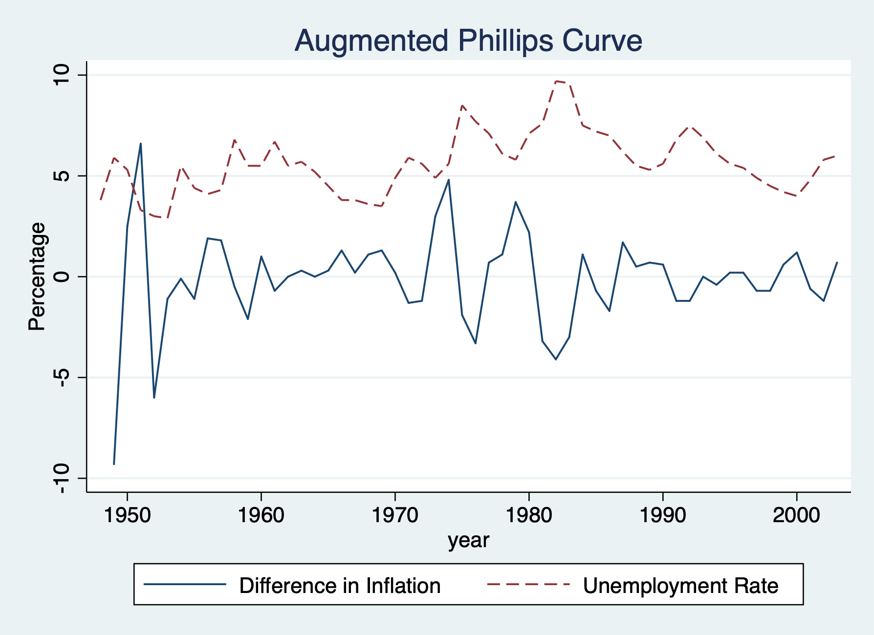
. twoway line cinf year || line unem year, lpattern(dash) ///
> legend(order(1 "Difference in Inflation" 2 "Unemployment Rate")) ///
> title("Augmented Phillips Curve") ytitle(Percentage) xtitle(year)
. graph export "week_10_augmented_phillips.png", replace
(file week_10_augmented_phillips.png written in PNG format)