Samuel Rowe - Adapted from Wooldridge and Mitchell
. clear

. set more off
Set Working Directory
. cd "/Users/Sam/Desktop/Econ 645/Data/Wooldridge"
/Users/Sam/Desktop/Econ 645/Data/Wooldridge
. use mroz.dta, clear
We’ll use the data from Mroz (1987) to look at the probability of a married woman being in the labor force. Labor force participation is a binary response. \[ y=[0,1] \] We will estimate the coefficients of the linear probability model (LPM), the logit estimator, and the probit estimator. Then, we’ll compare the marginal effects of all three estimators.
Summarize in the labor force
. tabulate inlf

       inlf │      Freq.     Percent        Cum.
────────────┼───────────────────────────────────
          0 │        325       43.16       43.16
          1 │        428       56.84      100.00
────────────┼───────────────────────────────────
      Total │        753      100.00
325 Women are not in the labor force and 428 Participating Our explanatory variables are non-wife income, education, experience, experience-squared, age, kids less than 6, kids greater than 6
. est clear
Logit
. eststo Logit: logit inlf nwifeinc educ exper expersq kidslt6 kidsge6

Iteration 0:   log likelihood =  -514.8732
Iteration 1:   log likelihood = -422.78042
Iteration 2:   log likelihood = -421.73851
Iteration 3:   log likelihood = -421.73502
Iteration 4:   log likelihood = -421.73502

Logistic regression                             Number of obs     =        753
                                                LR chi2(6)        =     186.28
                                                Prob > chi2       =     0.0000
Log likelihood = -421.73502                     Pseudo R2         =     0.1809

─────────────┬────────────────────────────────────────────────────────────────
        inlf │      Coef.   Std. Err.      z    P>|z|     [95% Conf. Interval]
─────────────┼────────────────────────────────────────────────────────────────
    nwifeinc │  -.0301171   .0082431    -3.65   0.000    -.0462734   -.0139609
        educ │   .2520038   .0425492     5.92   0.000      .168609    .3353987
       exper │   .2057387   .0310518     6.63   0.000     .1448784     .266599
     expersq │   -.003913   .0009994    -3.92   0.000    -.0058718   -.0019541
     kidslt6 │  -.9175126   .1742458    -5.27   0.000    -1.259028   -.5759971
     kidsge6 │   .2226164   .0683456     3.26   0.001     .0886616    .3565713
       _cons │  -3.739707    .543217    -6.88   0.000    -4.804392   -2.675021
─────────────┴────────────────────────────────────────────────────────────────
Probit
. eststo Probit: probit inlf nwifeinc educ exper expersq kidslt6 kidsge6

Iteration 0:   log likelihood =  -514.8732
Iteration 1:   log likelihood = -422.36847
Iteration 2:   log likelihood = -421.80202
Iteration 3:   log likelihood = -421.80161
Iteration 4:   log likelihood = -421.80161

Probit regression                               Number of obs     =        753
                                                LR chi2(6)        =     186.14
                                                Prob > chi2       =     0.0000
Log likelihood = -421.80161                     Pseudo R2         =     0.1808

─────────────┬────────────────────────────────────────────────────────────────
        inlf │      Coef.   Std. Err.      z    P>|z|     [95% Conf. Interval]
─────────────┼────────────────────────────────────────────────────────────────
    nwifeinc │   -.017188     .00474    -3.63   0.000    -.0264782   -.0078978
        educ │   .1501412     .02471     6.08   0.000     .1017105    .1985719
       exper │   .1240105   .0183233     6.77   0.000     .0880975    .1599236
     expersq │  -.0023694   .0005913    -4.01   0.000    -.0035284   -.0012103
     kidslt6 │  -.5543317   .1038244    -5.34   0.000    -.7578238   -.3508395
     kidsge6 │   .1307901   .0399186     3.28   0.001     .0525511    .2090292
       _cons │  -2.244553   .3146254    -7.13   0.000    -2.861207   -1.627899
─────────────┴────────────────────────────────────────────────────────────────
. esttab Logit Probit, mtitle

────────────────────────────────────────────
                      (1)             (2)
                    Logit          Probit
────────────────────────────────────────────
inlf
nwifeinc          -0.0301***      -0.0172***
                  (-3.65)         (-3.63)

educ                0.252***        0.150***
                   (5.92)          (6.08)

exper               0.206***        0.124***
                   (6.63)          (6.77)

expersq          -0.00391***     -0.00237***
                  (-3.92)         (-4.01)

kidslt6            -0.918***       -0.554***
                  (-5.27)         (-5.34)

kidsge6             0.223**         0.131**
                   (3.26)          (3.28)

_cons              -3.740***       -2.245***
                  (-6.88)         (-7.13)
────────────────────────────────────────────
N                     753             753
────────────────────────────────────────────
t statistics in parentheses
* p<0.05, ** p<0.01, *** p<0.001
. est clear
LPM
. quietly reg inlf nwifeinc educ exper expersq age kidslt6 kidsge6

. eststo LPM: margins, dydx(*) post

Average marginal effects                        Number of obs     =        753
Model VCE    : OLS

Expression   : Linear prediction, predict()
dy/dx w.r.t. : nwifeinc educ exper expersq age kidslt6 kidsge6

─────────────┬────────────────────────────────────────────────────────────────
             │            Delta-method
             │      dy/dx   Std. Err.      t    P>|t|     [95% Conf. Interval]
─────────────┼────────────────────────────────────────────────────────────────
    nwifeinc │  -.0034052   .0014485    -2.35   0.019    -.0062488   -.0005616
        educ │   .0379953    .007376     5.15   0.000      .023515    .0524756
       exper │   .0394924   .0056727     6.96   0.000     .0283561    .0506287
     expersq │  -.0005963   .0001848    -3.23   0.001    -.0009591   -.0002335
         age │  -.0160908   .0024847    -6.48   0.000    -.0209686    -.011213
     kidslt6 │  -.2618105   .0335058    -7.81   0.000    -.3275875   -.1960335
     kidsge6 │   .0130122    .013196     0.99   0.324    -.0128935    .0389179
─────────────┴────────────────────────────────────────────────────────────────
Logit
. quietly logit inlf nwifeinc educ exper expersq age kidslt6 kidsge6

. eststo Logit: margins, dydx(*) post

Average marginal effects                        Number of obs     =        753
Model VCE    : OIM

Expression   : Pr(inlf), predict()
dy/dx w.r.t. : nwifeinc educ exper expersq age kidslt6 kidsge6

─────────────┬────────────────────────────────────────────────────────────────
             │            Delta-method
             │      dy/dx   Std. Err.      z    P>|z|     [95% Conf. Interval]
─────────────┼────────────────────────────────────────────────────────────────
    nwifeinc │  -.0038118   .0014824    -2.57   0.010    -.0067172   -.0009064
        educ │   .0394965   .0072947     5.41   0.000     .0251992    .0537939
       exper │   .0367641     .00515     7.14   0.000     .0266702     .046858
     expersq │  -.0005633   .0001774    -3.18   0.001    -.0009109   -.0002156
         age │  -.0157194   .0023808    -6.60   0.000    -.0203856   -.0110532
     kidslt6 │  -.2577537   .0319416    -8.07   0.000    -.3203581   -.1951492
     kidsge6 │   .0107348    .013333     0.81   0.421    -.0153974    .0368671
─────────────┴────────────────────────────────────────────────────────────────
Probit
. quietly probit inlf nwifeinc educ exper expersq age kidslt6 kidsge6

. eststo Probit: margins, dydx(*) post

Average marginal effects                        Number of obs     =        753
Model VCE    : OIM

Expression   : Pr(inlf), predict()
dy/dx w.r.t. : nwifeinc educ exper expersq age kidslt6 kidsge6

─────────────┬────────────────────────────────────────────────────────────────
             │            Delta-method
             │      dy/dx   Std. Err.      z    P>|z|     [95% Conf. Interval]
─────────────┼────────────────────────────────────────────────────────────────
    nwifeinc │  -.0036162   .0014414    -2.51   0.012    -.0064413   -.0007911
        educ │   .0393703   .0072216     5.45   0.000     .0252161    .0535244
       exper │   .0370974   .0051522     7.20   0.000     .0269993    .0471956
     expersq │  -.0005675   .0001771    -3.20   0.001    -.0009146   -.0002204
         age │  -.0158957   .0023587    -6.74   0.000    -.0205186   -.0112728
     kidslt6 │  -.2611542   .0318597    -8.20   0.000    -.3235982   -.1987103
     kidsge6 │   .0108287   .0130584     0.83   0.407    -.0147654    .0364227
─────────────┴────────────────────────────────────────────────────────────────
. esttab LPM Logit Probit, mtitle

────────────────────────────────────────────────────────────
                      (1)             (2)             (3)
                      LPM           Logit          Probit
────────────────────────────────────────────────────────────
nwifeinc         -0.00341*       -0.00381*       -0.00362*
                  (-2.35)         (-2.57)         (-2.51)

educ               0.0380***       0.0395***       0.0394***
                   (5.15)          (5.41)          (5.45)

exper              0.0395***       0.0368***       0.0371***
                   (6.96)          (7.14)          (7.20)

expersq         -0.000596**     -0.000563**     -0.000568**
                  (-3.23)         (-3.18)         (-3.20)

age               -0.0161***      -0.0157***      -0.0159***
                  (-6.48)         (-6.60)         (-6.74)

kidslt6            -0.262***       -0.258***       -0.261***
                  (-7.81)         (-8.07)         (-8.20)

kidsge6            0.0130          0.0107          0.0108
                   (0.99)          (0.81)          (0.83)
────────────────────────────────────────────────────────────
N                     753             753             753
────────────────────────────────────────────────────────────
t statistics in parentheses
* p<0.05, ** p<0.01, *** p<0.001
. est clear
LPM
. quietly reg inlf nwifeinc educ exper expersq age kidslt6 kidsge6

. eststo LPM: margins, dydx(*) atmeans post

Conditional marginal effects                    Number of obs     =        753
Model VCE    : OLS

Expression   : Linear prediction, predict()
dy/dx w.r.t. : nwifeinc educ exper expersq age kidslt6 kidsge6
at           : nwifeinc        =    20.12896 (mean)
               educ            =    12.28685 (mean)
               exper           =    10.63081 (mean)
               expersq         =    178.0385 (mean)
               age             =    42.53785 (mean)
               kidslt6         =    .2377158 (mean)
               kidsge6         =    1.353254 (mean)

─────────────┬────────────────────────────────────────────────────────────────
             │            Delta-method
             │      dy/dx   Std. Err.      t    P>|t|     [95% Conf. Interval]
─────────────┼────────────────────────────────────────────────────────────────
    nwifeinc │  -.0034052   .0014485    -2.35   0.019    -.0062488   -.0005616
        educ │   .0379953    .007376     5.15   0.000      .023515    .0524756
       exper │   .0394924   .0056727     6.96   0.000     .0283561    .0506287
     expersq │  -.0005963   .0001848    -3.23   0.001    -.0009591   -.0002335
         age │  -.0160908   .0024847    -6.48   0.000    -.0209686    -.011213
     kidslt6 │  -.2618105   .0335058    -7.81   0.000    -.3275875   -.1960335
     kidsge6 │   .0130122    .013196     0.99   0.324    -.0128935    .0389179
─────────────┴────────────────────────────────────────────────────────────────
Logit
. quietly logit inlf nwifeinc educ exper expersq age kidslt6 kidsge6

. eststo Logit: margins, dydx(*) atmeans post

Conditional marginal effects                    Number of obs     =        753
Model VCE    : OIM

Expression   : Pr(inlf), predict()
dy/dx w.r.t. : nwifeinc educ exper expersq age kidslt6 kidsge6
at           : nwifeinc        =    20.12896 (mean)
               educ            =    12.28685 (mean)
               exper           =    10.63081 (mean)
               expersq         =    178.0385 (mean)
               age             =    42.53785 (mean)
               kidslt6         =    .2377158 (mean)
               kidsge6         =    1.353254 (mean)

─────────────┬────────────────────────────────────────────────────────────────
             │            Delta-method
             │      dy/dx   Std. Err.      z    P>|z|     [95% Conf. Interval]
─────────────┼────────────────────────────────────────────────────────────────
    nwifeinc │  -.0051901   .0020482    -2.53   0.011    -.0092045   -.0011756
        educ │   .0537773   .0105608     5.09   0.000     .0330785    .0744761
       exper │   .0500569   .0078247     6.40   0.000     .0347209     .065393
     expersq │  -.0007669   .0002477    -3.10   0.002    -.0012524   -.0002815
         age │   -.021403   .0035398    -6.05   0.000    -.0283408   -.0144652
     kidslt6 │  -.3509498   .0496395    -7.07   0.000    -.4482414   -.2536583
     kidsge6 │   .0146162   .0181884     0.80   0.422    -.0210324    .0502649
─────────────┴────────────────────────────────────────────────────────────────
Probit
. quietly probit inlf nwifeinc educ exper expersq age kidslt6 kidsge6

. eststo Probit: margins, dydx(*) atmeans post

Conditional marginal effects                    Number of obs     =        753
Model VCE    : OIM

Expression   : Pr(inlf), predict()
dy/dx w.r.t. : nwifeinc educ exper expersq age kidslt6 kidsge6
at           : nwifeinc        =    20.12896 (mean)
               educ            =    12.28685 (mean)
               exper           =    10.63081 (mean)
               expersq         =    178.0385 (mean)
               age             =    42.53785 (mean)
               kidslt6         =    .2377158 (mean)
               kidsge6         =    1.353254 (mean)

─────────────┬────────────────────────────────────────────────────────────────
             │            Delta-method
             │      dy/dx   Std. Err.      z    P>|z|     [95% Conf. Interval]
─────────────┼────────────────────────────────────────────────────────────────
    nwifeinc │  -.0046962   .0018903    -2.48   0.013    -.0084012   -.0009913
        educ │   .0511287   .0098592     5.19   0.000     .0318051    .0704523
       exper │   .0481771   .0073278     6.57   0.000     .0338149    .0625392
     expersq │  -.0007371   .0002347    -3.14   0.002     -.001197   -.0002771
         age │  -.0206432   .0033079    -6.24   0.000    -.0271265   -.0141598
     kidslt6 │  -.3391514   .0463581    -7.32   0.000    -.4300117   -.2482911
     kidsge6 │   .0140628   .0169852     0.83   0.408    -.0192275    .0473531
─────────────┴────────────────────────────────────────────────────────────────
Compare
. esttab LPM Logit Probit, mtitle

────────────────────────────────────────────────────────────
                      (1)             (2)             (3)
                      LPM           Logit          Probit
────────────────────────────────────────────────────────────
nwifeinc         -0.00341*       -0.00519*       -0.00470*
                  (-2.35)         (-2.53)         (-2.48)

educ               0.0380***       0.0538***       0.0511***
                   (5.15)          (5.09)          (5.19)

exper              0.0395***       0.0501***       0.0482***
                   (6.96)          (6.40)          (6.57)

expersq         -0.000596**     -0.000767**     -0.000737**
                  (-3.23)         (-3.10)         (-3.14)

age               -0.0161***      -0.0214***      -0.0206***
                  (-6.48)         (-6.05)         (-6.24)

kidslt6            -0.262***       -0.351***       -0.339***
                  (-7.81)         (-7.07)         (-7.32)

kidsge6            0.0130          0.0146          0.0141
                   (0.99)          (0.80)          (0.83)
────────────────────────────────────────────────────────────
N                     753             753             753
────────────────────────────────────────────────────────────
t statistics in parentheses
* p<0.05, ** p<0.01, *** p<0.001
The analysis shows that the marginal effects are fairly close across the linear probability model, Logit model, and Probit model. One additional year of education increases the probability of being in the labor force by a range of 0.038 to 0.0395 percentage points. Interestingly, one additional child less than six is associated with a drop in the probability of being in the labor force by a range of 0.258 to 0.262.
Please not that around the means, our linear probability model, Logit, and Probit should be fairly similar. However, the marginal effects for the linear probability model are constant and will not vary across different values of x.
We can use the option, or to get odds ratios after running a logit.
\[ OR = \frac{(Odds Success)}{(Odds Failure)} = \frac{p(1)/(1-p(1))}{p(0)/(1-p(0))} \]
. logit inlf nwifeinc educ exper expersq age kidslt6 kidsge6, or

Iteration 0:   log likelihood =  -514.8732
Iteration 1:   log likelihood = -402.38502
Iteration 2:   log likelihood = -401.76569
Iteration 3:   log likelihood = -401.76515
Iteration 4:   log likelihood = -401.76515

Logistic regression                             Number of obs     =        753
                                                LR chi2(7)        =     226.22
                                                Prob > chi2       =     0.0000
Log likelihood = -401.76515                     Pseudo R2         =     0.2197

─────────────┬────────────────────────────────────────────────────────────────
        inlf │ Odds Ratio   Std. Err.      z    P>|z|     [95% Conf. Interval]
─────────────┼────────────────────────────────────────────────────────────────
    nwifeinc │    .978881   .0082436    -2.53   0.011     .9628565    .9951723
        educ │   1.247536   .0541925     5.09   0.000     1.145717    1.358404
       exper │   1.228593   .0393849     6.42   0.000     1.153775    1.308263
     expersq │   .9968509   .0010129    -3.10   0.002     .9948676    .9988381
         age │   .9157386   .0133451    -6.04   0.000     .8899527    .9422715
     kidslt6 │   .2361344   .0480734    -7.09   0.000      .158441    .3519257
     kidsge6 │   1.061956   .0794234     0.80   0.422     .9171603     1.22961
       _cons │   1.530283   1.316609     0.49   0.621     .2834155    8.262655
─────────────┴────────────────────────────────────────────────────────────────
One additional year of education is associated with a 1.25 times increase in the odds of being in the labor force (or an increase of 25%) holding all other variables constant. One additional child less than six decreases the odds of being in the labor force by a factor of 0.24 holding all other variables constant (or a decrease of 76%).
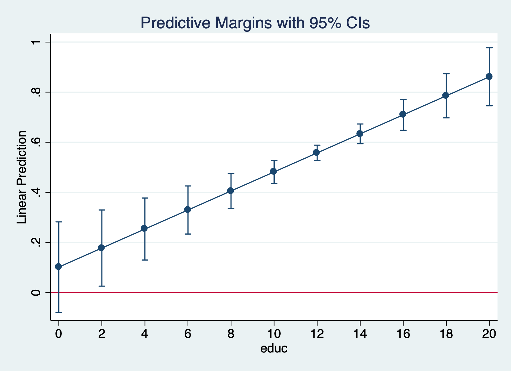
LPM
. est clear

. quietly reg inlf nwifeinc educ exper expersq age kidslt6 kidsge6

. eststo lpm: margins, at(educ=(0(2)20)) post

Predictive margins                              Number of obs     =        753
Model VCE    : OLS

Expression   : Linear prediction, predict()

1._at        : educ            =           0

2._at        : educ            =           2

3._at        : educ            =           4

4._at        : educ            =           6

5._at        : educ            =           8

6._at        : educ            =          10

7._at        : educ            =          12

8._at        : educ            =          14

9._at        : educ            =          16

10._at       : educ            =          18

11._at       : educ            =          20

─────────────┬────────────────────────────────────────────────────────────────
             │            Delta-method
             │     Margin   Std. Err.      t    P>|t|     [95% Conf. Interval]
─────────────┼────────────────────────────────────────────────────────────────
         _at │
          1  │   .1015504    .091955     1.10   0.270    -.0789714    .2820723
          2  │    .177541   .0774562     2.29   0.022     .0254827    .3295993
          3  │   .2535316   .0630748     4.02   0.000     .1297062    .3773571
          4  │   .3295222   .0489147     6.74   0.000     .2334952    .4255492
          5  │   .4055128   .0352435    11.51   0.000     .3363244    .4747013
          6  │   .4815034   .0229524    20.98   0.000     .4364444    .5265625
          7  │    .557494   .0157087    35.49   0.000     .5266554    .5883327
          8  │   .6334846    .020049    31.60   0.000     .5941254    .6728439
          9  │   .7094753   .0315024    22.52   0.000     .6476311    .7713194
         10  │   .7854659   .0449232    17.48   0.000     .6972748    .8736569
         11  │   .8614565   .0589832    14.61   0.000     .7456633    .9772496
─────────────┴────────────────────────────────────────────────────────────────

. marginsplot, yline(0)

  Variables that uniquely identify margins: educ
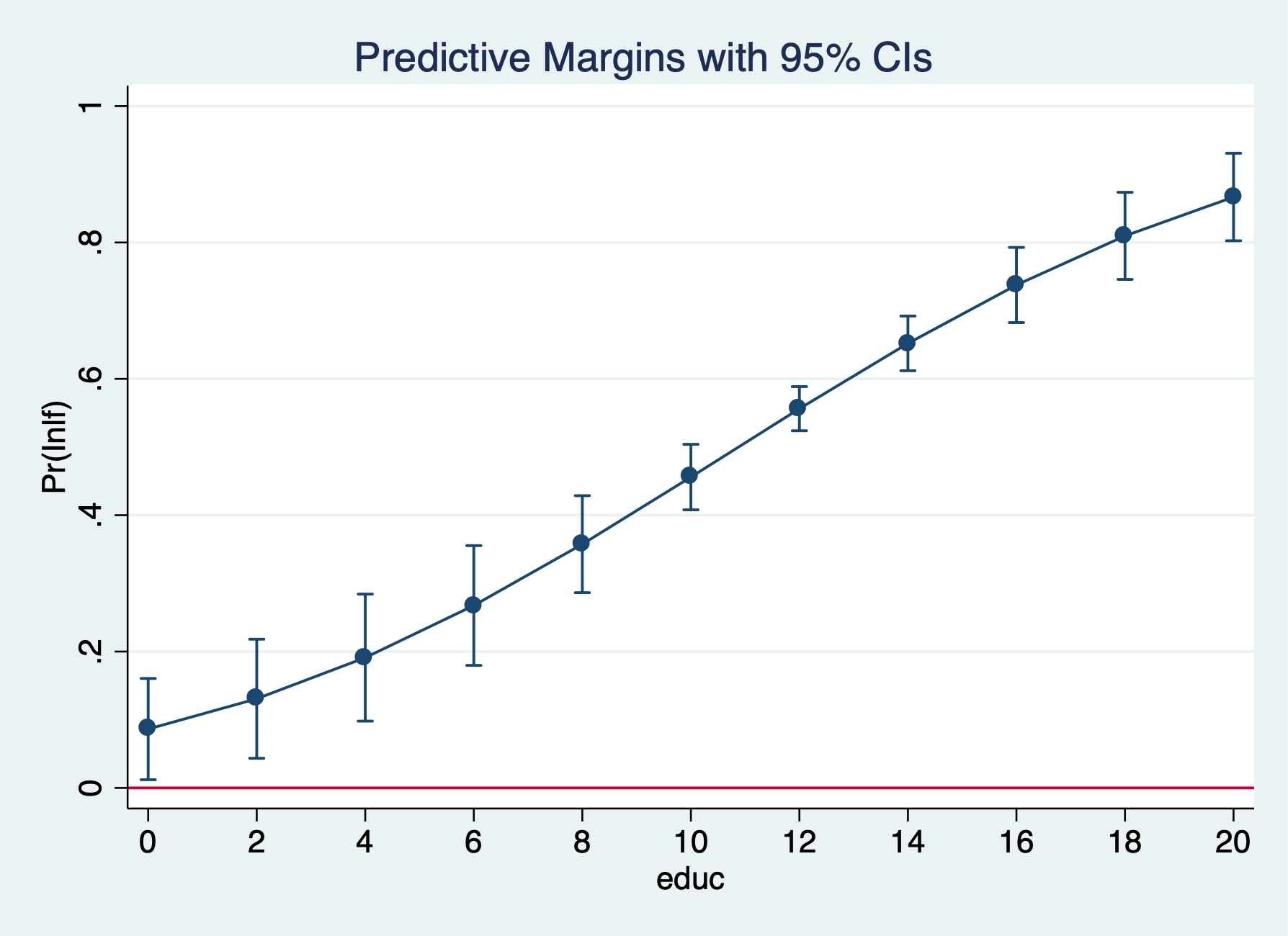
Logit
. quietly logit inlf nwifeinc educ exper expersq kidslt6 kidsge6

. eststo logit1: margins, at(educ=(0(2)20)) post

Predictive margins                              Number of obs     =        753
Model VCE    : OIM

Expression   : Pr(inlf), predict()

1._at        : educ            =           0

2._at        : educ            =           2

3._at        : educ            =           4

4._at        : educ            =           6

5._at        : educ            =           8

6._at        : educ            =          10

7._at        : educ            =          12

8._at        : educ            =          14

9._at        : educ            =          16

10._at       : educ            =          18

11._at       : educ            =          20

─────────────┬────────────────────────────────────────────────────────────────
             │            Delta-method
             │     Margin   Std. Err.      z    P>|z|     [95% Conf. Interval]
─────────────┼────────────────────────────────────────────────────────────────
         _at │
          1  │   .0862997   .0378791     2.28   0.023     .0120581    .1605413
          2  │   .1307839     .04457     2.93   0.003     .0434283    .2181396
          3  │   .1911164   .0475215     4.02   0.000      .097976    .2842567
          4  │   .2675469   .0448132     5.97   0.000     .1797146    .3553791
          5  │   .3575117   .0362904     9.85   0.000     .2863838    .4286396
          6  │    .455911    .024513    18.60   0.000     .4078663    .5039556
          7  │   .5562468   .0165243    33.66   0.000     .5238597    .5886338
          8  │   .6519779   .0204676    31.85   0.000     .6118622    .6920936
          9  │   .7376484   .0281232    26.23   0.000     .6825279    .7927688
         10  │   .8096698   .0325919    24.84   0.000     .7457909    .8735486
         11  │   .8666826   .0327653    26.45   0.000     .8024638    .9309015
─────────────┴────────────────────────────────────────────────────────────────

. marginsplot, yline(0)

  Variables that uniquely identify margins: educ
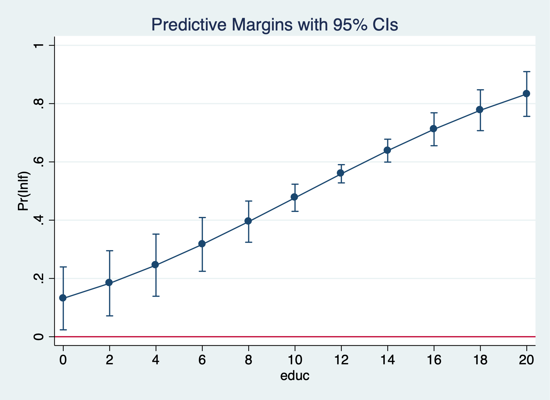
Probit
. quietly probit inlf nwifeinc educ exper expersq age kidslt6 kidsge6

. eststo probit1: margins, at(educ=(0(2)20)) post

Predictive margins                              Number of obs     =        753
Model VCE    : OIM

Expression   : Pr(inlf), predict()

1._at        : educ            =           0

2._at        : educ            =           2

3._at        : educ            =           4

4._at        : educ            =           6

5._at        : educ            =           8

6._at        : educ            =          10

7._at        : educ            =          12

8._at        : educ            =          14

9._at        : educ            =          16

10._at       : educ            =          18

11._at       : educ            =          20

─────────────┬────────────────────────────────────────────────────────────────
             │            Delta-method
             │     Margin   Std. Err.      z    P>|z|     [95% Conf. Interval]
─────────────┼────────────────────────────────────────────────────────────────
         _at │
          1  │   .1315922    .055059     2.39   0.017     .0236785    .2395059
          2  │   .1833441   .0570249     3.22   0.001     .0715773    .2951109
          3  │   .2455272   .0543798     4.52   0.000     .1389447    .3521097
          4  │   .3168216   .0470756     6.73   0.000     .2245552     .409088
          5  │   .3949415   .0360827    10.95   0.000     .3242206    .4656623
          6  │   .4768675   .0237722    20.06   0.000     .4302749    .5234602
          7  │   .5592018   .0159547    35.05   0.000     .5279311    .5904724
          8  │   .6385748   .0200316    31.88   0.000     .5993136     .677836
          9  │   .7120285   .0288142    24.71   0.000     .6555538    .7685032
         10  │   .7773109   .0357596    21.74   0.000     .7072234    .8473984
         11  │   .8330432   .0391944    21.25   0.000     .7562235    .9098629
─────────────┴────────────────────────────────────────────────────────────────

. marginsplot, yline(0)

  Variables that uniquely identify margins: educ
The predicted probability that a married women is in the labor force rises from 47.7% for 12 years of education to 71.2% for 16 years of education.
. coefplot lpm logit1, at recast(line) ciopts(recast(rline) lpattern(dash))

. coefplot lpm probit1, at recast(line) ciopts(recast(rline) lpattern(dash))

. coefplot logit1 probit1, at recast(line) ciopts(recast(rline) lpattern(dash))
LPM
. quietly reg inlf nwifeinc educ exper expersq age kidslt6 kidsge6

. margins, dydx(kidslt6) at(educ=(0(2)20))

Average marginal effects                        Number of obs     =        753
Model VCE    : OLS

Expression   : Linear prediction, predict()
dy/dx w.r.t. : kidslt6

1._at        : educ            =           0

2._at        : educ            =           2

3._at        : educ            =           4

4._at        : educ            =           6

5._at        : educ            =           8

6._at        : educ            =          10

7._at        : educ            =          12

8._at        : educ            =          14

9._at        : educ            =          16

10._at       : educ            =          18

11._at       : educ            =          20

─────────────┬────────────────────────────────────────────────────────────────
             │            Delta-method
             │      dy/dx   Std. Err.      t    P>|t|     [95% Conf. Interval]
─────────────┼────────────────────────────────────────────────────────────────
kidslt6      │
         _at │
          1  │  -.2618105   .0335058    -7.81   0.000    -.3275875   -.1960335
          2  │  -.2618105   .0335058    -7.81   0.000    -.3275875   -.1960335
          3  │  -.2618105   .0335058    -7.81   0.000    -.3275875   -.1960335
          4  │  -.2618105   .0335058    -7.81   0.000    -.3275875   -.1960335
          5  │  -.2618105   .0335058    -7.81   0.000    -.3275875   -.1960335
          6  │  -.2618105   .0335058    -7.81   0.000    -.3275875   -.1960335
          7  │  -.2618105   .0335058    -7.81   0.000    -.3275875   -.1960335
          8  │  -.2618105   .0335058    -7.81   0.000    -.3275875   -.1960335
          9  │  -.2618105   .0335058    -7.81   0.000    -.3275875   -.1960335
         10  │  -.2618105   .0335058    -7.81   0.000    -.3275875   -.1960335
         11  │  -.2618105   .0335058    -7.81   0.000    -.3275875   -.1960335
─────────────┴────────────────────────────────────────────────────────────────

. marginsplot, yline(0)

  Variables that uniquely identify margins: educ
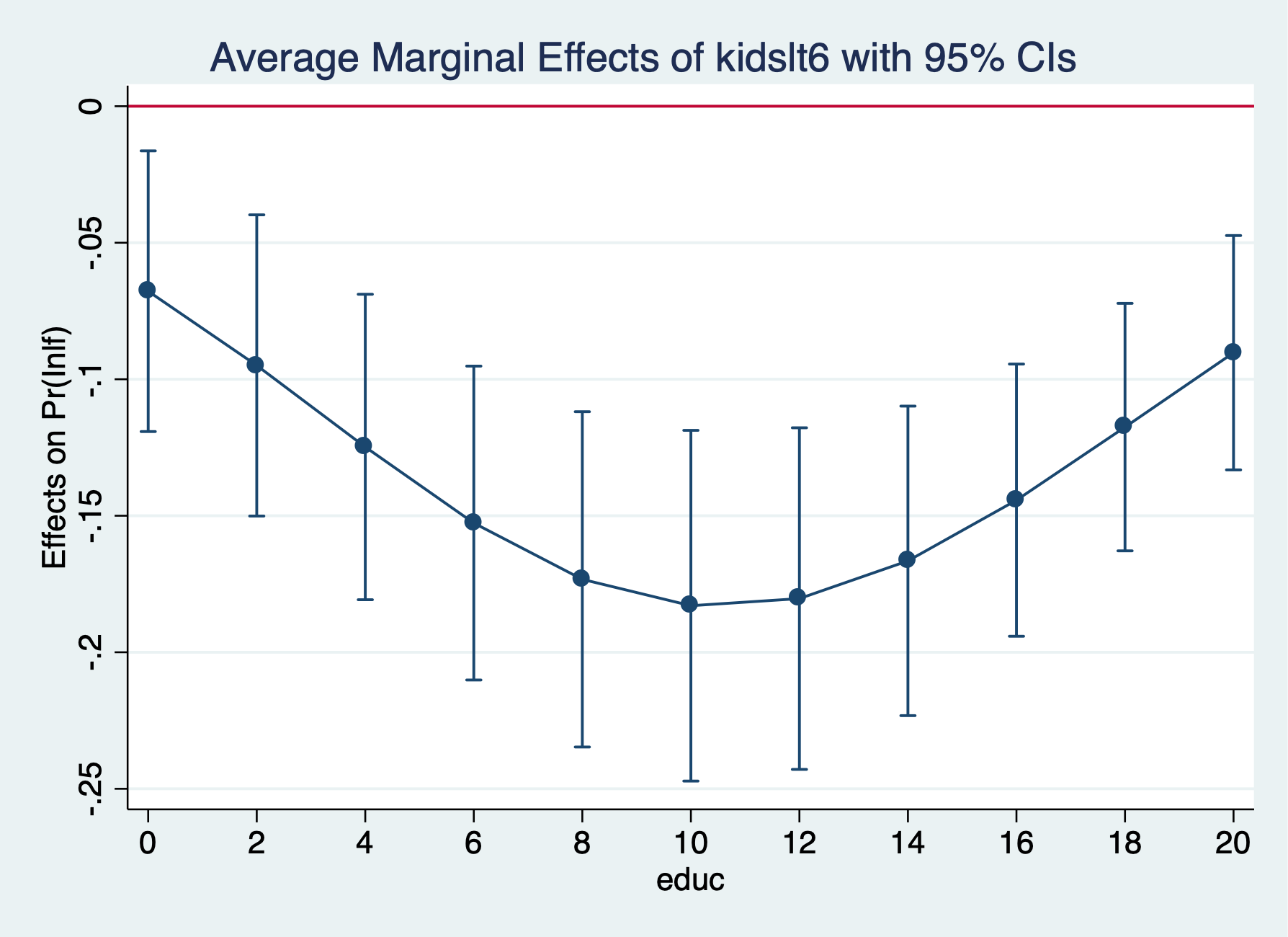
Logit
. quietly logit inlf nwifeinc educ exper expersq kidslt6 kidsge6

. margins, dydx(kidslt6) at(educ=(0(2)20))

Average marginal effects                        Number of obs     =        753
Model VCE    : OIM

Expression   : Pr(inlf), predict()
dy/dx w.r.t. : kidslt6

1._at        : educ            =           0

2._at        : educ            =           2

3._at        : educ            =           4

4._at        : educ            =           6

5._at        : educ            =           8

6._at        : educ            =          10

7._at        : educ            =          12

8._at        : educ            =          14

9._at        : educ            =          16

10._at       : educ            =          18

11._at       : educ            =          20

─────────────┬────────────────────────────────────────────────────────────────
             │            Delta-method
             │      dy/dx   Std. Err.      z    P>|z|     [95% Conf. Interval]
─────────────┼────────────────────────────────────────────────────────────────
kidslt6      │
         _at │
          1  │  -.0677567   .0262236    -2.58   0.010    -.1191539   -.0163594
          2  │  -.0949468   .0281434    -3.37   0.001    -.1501069   -.0397867
          3  │  -.1248173   .0285395    -4.37   0.000    -.1807537   -.0688808
          4  │  -.1526688   .0293293    -5.21   0.000    -.2101531   -.0951844
          5  │  -.1732958   .0313347    -5.53   0.000    -.2347106    -.111881
          6  │  -.1829484   .0327734    -5.58   0.000    -.2471831   -.1187137
          7  │  -.1803418   .0319215    -5.65   0.000    -.2429069   -.1177768
          8  │  -.1665232   .0289231    -5.76   0.000    -.2232115   -.1098349
          9  │  -.1442912   .0254362    -5.67   0.000    -.1941452   -.0944372
         10  │  -.1175221   .0231237    -5.08   0.000    -.1628437   -.0722005
         11  │  -.0902871   .0218973    -4.12   0.000    -.1332051   -.0473691
─────────────┴────────────────────────────────────────────────────────────────

. marginsplot, yline(0)

  Variables that uniquely identify margins: educ

. graph export "/Users/Sam/Desktop/Econ 645/Stata/week8_logitinlf.png", replace
(file /Users/Sam/Desktop/Econ 645/Stata/week8_logitinlf.png written in PNG format)
Probit
. quietly probit inlf nwifeinc educ exper expersq age kidslt6 kidsge6

. margins, dydx(kidslt6) at(educ=(0(2)20))

Average marginal effects                        Number of obs     =        753
Model VCE    : OIM

Expression   : Pr(inlf), predict()
dy/dx w.r.t. : kidslt6

1._at        : educ            =           0

2._at        : educ            =           2

3._at        : educ            =           4

4._at        : educ            =           6

5._at        : educ            =           8

6._at        : educ            =          10

7._at        : educ            =          12

8._at        : educ            =          14

9._at        : educ            =          16

10._at       : educ            =          18

11._at       : educ            =          20

─────────────┬────────────────────────────────────────────────────────────────
             │            Delta-method
             │      dy/dx   Std. Err.      z    P>|z|     [95% Conf. Interval]
─────────────┼────────────────────────────────────────────────────────────────
kidslt6      │
         _at │
          1  │   -.153748   .0455045    -3.38   0.001    -.2429352   -.0645607
          2  │  -.1893831   .0408614    -4.63   0.000    -.2694699   -.1092962
          3  │  -.2223621   .0360335    -6.17   0.000    -.2929864   -.1517377
          4  │  -.2492771    .033371    -7.47   0.000    -.3146829   -.1838712
          5  │  -.2672253   .0331963    -8.05   0.000    -.3322889   -.2021617
          6  │  -.2743121   .0335951    -8.17   0.000    -.3401572    -.208467
          7  │  -.2699501    .032832    -8.22   0.000    -.3342997   -.2056006
          8  │   -.254902    .030869    -8.26   0.000    -.3154042   -.1943998
          9  │  -.2310833   .0292123    -7.91   0.000    -.2883384   -.1738282
         10  │  -.2011899   .0295232    -6.81   0.000    -.2590542   -.1433256
         11  │  -.1682404   .0317255    -5.30   0.000    -.2304211   -.1060596
─────────────┴────────────────────────────────────────────────────────────────

. marginsplot, yline(0)

  Variables that uniquely identify margins: educ
The average marginal effect for an additional child less than 6 rises from -18.3 percentage points to -14.4 percentage points, but the difference does not appear to be statistically significant.
. use "/Users/Sam/Desktop/Econ 645/Data/CPS/mlogit_example.dta", clear
Our multinominal logit model
We will use Current Population Survey Data from September 2023 and 2024 to estimate the following model for labor force participation: \[ lfs_{i}=\beta_{0}+\beta_1 edu_{i} + \beta_2 exper_i + ... + u_i \]. There are three alternatives: Employed, Unemployed, and Not in the Labor Force.
. tab laborforce

Labor Force │
     Status │      Freq.     Percent        Cum.
────────────┼───────────────────────────────────
   Employed │     23,760       57.12       57.12
 Unemployed │        832        2.00       59.12
       NILF │     17,007       40.88      100.00
────────────┼───────────────────────────────────
      Total │     41,599      100.00

. tab laborforce, nolabel

Labor Force │
     Status │      Freq.     Percent        Cum.
────────────┼───────────────────────────────────
          1 │     23,760       57.12       57.12
          2 │        832        2.00       59.12
          3 │     17,007       40.88      100.00
────────────┼───────────────────────────────────
      Total │     41,599      100.00
Our dependent variable has three nominal categories. \[ y=[1,2,3] \] оr \[ y=[Employed, Unemployed, NILF] \]
We use the mlogit command to run a multinomial logit to get log odds for J-1 logits.
. mlogit laborforce i.educat exp exp2 i.race_ethnicity i.female i.metroarea i.union i.marital i.hryear4

Iteration 0:   log likelihood = -31774.039
Iteration 1:   log likelihood = -22975.759
Iteration 2:   log likelihood = -22620.368
Iteration 3:   log likelihood = -22573.244
Iteration 4:   log likelihood = -22565.789
Iteration 5:   log likelihood = -22564.343
Iteration 6:   log likelihood = -22564.014
Iteration 7:   log likelihood = -22563.941
Iteration 8:   log likelihood = -22563.925
Iteration 9:   log likelihood = -22563.922
Iteration 10:  log likelihood = -22563.922
Iteration 11:  log likelihood = -22563.922
Iteration 12:  log likelihood = -22563.922

Multinomial logistic regression                 Number of obs     =     41,599
                                                LR chi2(38)       =   18420.23
                                                Prob > chi2       =     0.0000
Log likelihood = -22563.922                     Pseudo R2         =     0.2899

──────────────────────────┬────────────────────────────────────────────────────────────────
         laborforcestatus │      Coef.   Std. Err.      z    P>|z|     [95% Conf. Interval]
──────────────────────────┼────────────────────────────────────────────────────────────────
Employed                  │  (base outcome)
──────────────────────────┼────────────────────────────────────────────────────────────────
Unemployed                │
                   educat │
                     HSD  │  -.2279524   .1119685    -2.04   0.042    -.4474066   -.0084982
            Some College  │  -.4312492   .1303621    -3.31   0.001    -.6867542   -.1757442
           AA/Vocational  │  -.6931682    .165487    -4.19   0.000    -1.017517   -.3688197
                   BS/BA  │  -.6706784   .1331892    -5.04   0.000    -.9317245   -.4096323
Graduate or Professional  │  -1.063383   .1745188    -6.09   0.000    -1.405433   -.7213323
                          │
                      exp │  -.0291051   .0088759    -3.28   0.001    -.0465016   -.0117087
                     exp2 │   .0002524   .0001575     1.60   0.109    -.0000562    .0005611
                          │
           race_ethnicity │
  Asian/Pacific Islander  │   -.813795   .3012644    -2.70   0.007    -1.404262   -.2233275
                   Black  │  -.3951124   .2756281    -1.43   0.152    -.9353337    .1451088
         Hispanic/Latino  │  -.6504449   .2691511    -2.42   0.016    -1.177971   -.1229184
                   White  │  -.7855686   .2616547    -3.00   0.003    -1.298402   -.2727347
             Multiracial  │  -.4798449   .3366208    -1.43   0.154     -1.13961    .1799197
                          │
                   female │
                  Female  │  -.0004137   .0721979    -0.01   0.995     -.141919    .1410915
                          │
                metroarea │
           Nonmetro Area  │  -.1010417    .097797    -1.03   0.302    -.2927204    .0906369
          Not Identified  │   .0635435    .346152     0.18   0.854     -.614902     .741989
                          │
                    union │
                   Union  │  -19.66515   2339.277    -0.01   0.993    -4604.564    4565.234
                          │
                  marital │
    Divorced/Sep/Widowed  │   .6132556   .1175463     5.22   0.000     .3828691     .843642
           Never Married  │   .7526873   .0988405     7.62   0.000     .5589634    .9464112
                          │
                  hryear4 │
                    2024  │   .0228376    .071126     0.32   0.748    -.1165667    .1622419
                          │
                    _cons │  -2.023219   .3012462    -6.72   0.000    -2.613651   -1.432787
──────────────────────────┼────────────────────────────────────────────────────────────────
NILF                      │
                   educat │
                     HSD  │  -.7898216   .0425444   -18.56   0.000    -.8732071   -.7064361
            Some College  │  -.8941042   .0479568   -18.64   0.000    -.9880978   -.8001105
           AA/Vocational  │  -1.143176   .0559087   -20.45   0.000    -1.252755   -1.033597
                   BS/BA  │  -1.493236   .0488335   -30.58   0.000    -1.588948   -1.397524
Graduate or Professional  │  -1.746904   .0561914   -31.09   0.000    -1.857038   -1.636771
                          │
                      exp │  -.1490983    .003087   -48.30   0.000    -.1551487    -.143048
                     exp2 │   .0031412   .0000469    66.92   0.000     .0030492    .0032332
                          │
           race_ethnicity │
  Asian/Pacific Islander  │  -.1995846   .1336975    -1.49   0.135    -.4616269    .0624578
                   Black  │  -.1053158   .1293382    -0.81   0.415     -.358814    .1481824
         Hispanic/Latino  │  -.4785722   .1270357    -3.77   0.000    -.7275575   -.2295869
                   White  │  -.3378929   .1237786    -2.73   0.006    -.5804944   -.0952913
             Multiracial  │  -.1802636   .1537778    -1.17   0.241    -.4816625    .1211354
                          │
                   female │
                  Female  │   .5781835   .0258942    22.33   0.000     .5274318    .6289351
                          │
                metroarea │
           Nonmetro Area  │  -.0069684   .0328081    -0.21   0.832    -.0712712    .0573344
          Not Identified  │  -.0021328   .1282129    -0.02   0.987    -.2534254    .2491598
                          │
                    union │
                   Union  │  -20.25621   566.9973    -0.04   0.972     -1131.55    1091.038
                          │
                  marital │
    Divorced/Sep/Widowed  │  -.0531382   .0373157    -1.42   0.154    -.1262757    .0199993
           Never Married  │   .1464745   .0379587     3.86   0.000     .0720769    .2208722
                          │
                  hryear4 │
                    2024  │  -.0398405   .0253899    -1.57   0.117    -.0896037    .0099228
                          │
                    _cons │   1.072448   .1365064     7.86   0.000     .8049003    1.339996
──────────────────────────┴────────────────────────────────────────────────────────────────
Note: 2044 observations completely determined.  Standard errors questionable.
Next, we need to test our Independence of Irrelevant Alternatives (IIA) assumption with a Hausman Test.
Estimate an Unrestricted model - We’ll remove unemployed
. quietly mlogit laborforce i.educat exp exp2 i.race_ethnicity i.female i.metroarea i.union i.marital i.hryear4

. estimates store unrestricted
We compare the log odds for unemployed and not in the labor force to being employed. Given that these are log odds, we’ll need to convert them to Odds Ratios or find the marginal effects.
Estimate a Restricted Model to test Independence of Irrelevant Alternatives assumption
. quietly mlogit laborforce i.educat exp exp2 i.race_ethnicity i.female i.metroarea i.union i.marital if laborforce
>  !=2

. estimate store restricted
Use hausman command
. hausman restricted unrestricted, alleqs constant

Note: the rank of the differenced variance matrix (2) does not equal the number of coefficients being tested (19);
        be sure this is what you expect, or there may be problems computing the test.  Examine the output of your
        estimators for anything unexpected and possibly consider scaling your variables so that the coefficients
        are on a similar scale.

                 ──── Coefficients ────
             │      (b)          (B)            (b-B)     sqrt(diag(V_b-V_B))
             │   restricted  unrestricted    Difference          S.E.
─────────────┼────────────────────────────────────────────────────────────────
      educat │
          2  │   -.7860864    -.7898216        .0037352        .0035785
          3  │     -.89149    -.8941042        .0026142        .0032032
          4  │   -1.140012    -1.143176         .003164         .003669
          5  │   -1.486705    -1.493236        .0065306        .0036976
          6  │   -1.737118    -1.746904        .0097867        .0035815
         exp │   -.1486206    -.1490983        .0004777        .0002218
        exp2 │    .0031335     .0031412       -7.78e-06        2.91e-06
race_ethni~y │
          2  │   -.1712505    -.1995846        .0283341        .0120289
          3  │   -.0717454    -.1053158        .0335704        .0121412
          4  │   -.4427331    -.4785722        .0358391        .0115676
          5  │   -.3060009    -.3378929         .031892        .0117006
          6  │   -.1491388    -.1802636        .0311247        .0136923
    1.female │    .5793374     .5781835        .0011539        .0018992
   metroarea │
          2  │   -.0070074    -.0069684        -.000039         .002025
          3  │   -.0064057    -.0021328       -.0042729        .0112617
     1.union │   -20.20846    -20.25621        .0477553               .
     marital │
          2  │   -.0524486    -.0531382        .0006896        .0022895
          3  │    .1495841     .1464745        .0031096        .0023193
       _cons │     1.00979     1.072448       -.0626578               .
─────────────┴────────────────────────────────────────────────────────────────
                          b = consistent under Ho and Ha; obtained from mlogit
           B = inconsistent under Ha, efficient under Ho; obtained from mlogit

    Test:  Ho:  difference in coefficients not systematic

                  chi2(2) = (b-B)'[(V_b-V_B)^(-1)](b-B)
                          =        8.92
                Prob>chi2 =      0.0116
                (V_b-V_B is not positive definite)
Our chi-squared is 8.92, which means with reject the IIA assumption. We should consider a binary response here.
Next, we use Stata to estimate predicted probabilities
. quietly mlogit laborforce i.educat exp exp2 i.race_ethnicity i.female i.metroarea i.union i.marital, base(1)

. margins, atmeans predict(outcome(1))

Adjusted predictions                            Number of obs     =     41,599
Model VCE    : OIM

Expression   : Pr(laborforcestatus==Employed), predict(outcome(1))
at           : 1.educat        =    .1261088 (mean)
               2.educat        =     .286954 (mean)
               3.educat        =    .1488497 (mean)
               4.educat        =    .0969254 (mean)
               5.educat        =    .2079617 (mean)
               6.educat        =    .1332003 (mean)
               exp             =    32.89247 (mean)
               exp2            =    1467.595 (mean)
               1.race_eth~y    =    .0098079 (mean)
               2.race_eth~y    =    .0622611 (mean)
               3.race_eth~y    =    .0931032 (mean)
               4.race_eth~y    =    .1487776 (mean)
               5.race_eth~y    =    .6685738 (mean)
               6.race_eth~y    =    .0174764 (mean)
               0.female        =    .4804923 (mean)
               1.female        =    .5195077 (mean)
               1.metroarea     =    .8000673 (mean)
               2.metroarea     =    .1904132 (mean)
               3.metroarea     =    .0095195 (mean)
               0.union         =    .9508642 (mean)
               1.union         =    .0491358 (mean)
               1.marital       =    .5163586 (mean)
               2.marital       =    .1819515 (mean)
               3.marital       =    .3016899 (mean)

─────────────┬────────────────────────────────────────────────────────────────
             │            Delta-method
             │     Margin   Std. Err.      z    P>|z|     [95% Conf. Interval]
─────────────┼────────────────────────────────────────────────────────────────
       _cons │   .7684672   4.830264     0.16   0.874    -8.698677    10.23561
─────────────┴────────────────────────────────────────────────────────────────

. margins, atmeans predict(outcome(2))

Adjusted predictions                            Number of obs     =     41,599
Model VCE    : OIM

Expression   : Pr(laborforcestatus==Unemployed), predict(outcome(2))
at           : 1.educat        =    .1261088 (mean)
               2.educat        =     .286954 (mean)
               3.educat        =    .1488497 (mean)
               4.educat        =    .0969254 (mean)
               5.educat        =    .2079617 (mean)
               6.educat        =    .1332003 (mean)
               exp             =    32.89247 (mean)
               exp2            =    1467.595 (mean)
               1.race_eth~y    =    .0098079 (mean)
               2.race_eth~y    =    .0622611 (mean)
               3.race_eth~y    =    .0931032 (mean)
               4.race_eth~y    =    .1487776 (mean)
               5.race_eth~y    =    .6685738 (mean)
               6.race_eth~y    =    .0174764 (mean)
               0.female        =    .4804923 (mean)
               1.female        =    .5195077 (mean)
               1.metroarea     =    .8000673 (mean)
               2.metroarea     =    .1904132 (mean)
               3.metroarea     =    .0095195 (mean)
               0.union         =    .9508642 (mean)
               1.union         =    .0491358 (mean)
               1.marital       =    .5163586 (mean)
               2.marital       =    .1819515 (mean)
               3.marital       =    .3016899 (mean)

─────────────┬────────────────────────────────────────────────────────────────
             │            Delta-method
             │     Margin   Std. Err.      z    P>|z|     [95% Conf. Interval]
─────────────┼────────────────────────────────────────────────────────────────
       _cons │   .0090578    1.03352     0.01   0.993    -2.016605     2.03472
─────────────┴────────────────────────────────────────────────────────────────

. margins, atmeans predict(outcome(3))

Adjusted predictions                            Number of obs     =     41,599
Model VCE    : OIM

Expression   : Pr(laborforcestatus==NILF), predict(outcome(3))
at           : 1.educat        =    .1261088 (mean)
               2.educat        =     .286954 (mean)
               3.educat        =    .1488497 (mean)
               4.educat        =    .0969254 (mean)
               5.educat        =    .2079617 (mean)
               6.educat        =    .1332003 (mean)
               exp             =    32.89247 (mean)
               exp2            =    1467.595 (mean)
               1.race_eth~y    =    .0098079 (mean)
               2.race_eth~y    =    .0622611 (mean)
               3.race_eth~y    =    .0931032 (mean)
               4.race_eth~y    =    .1487776 (mean)
               5.race_eth~y    =    .6685738 (mean)
               6.race_eth~y    =    .0174764 (mean)
               0.female        =    .4804923 (mean)
               1.female        =    .5195077 (mean)
               1.metroarea     =    .8000673 (mean)
               2.metroarea     =    .1904132 (mean)
               3.metroarea     =    .0095195 (mean)
               0.union         =    .9508642 (mean)
               1.union         =    .0491358 (mean)
               1.marital       =    .5163586 (mean)
               2.marital       =    .1819515 (mean)
               3.marital       =    .3016899 (mean)

─────────────┬────────────────────────────────────────────────────────────────
             │            Delta-method
             │     Margin   Std. Err.      z    P>|z|     [95% Conf. Interval]
─────────────┼────────────────────────────────────────────────────────────────
       _cons │   .2224751   4.825216     0.05   0.963    -9.234774    9.679725
─────────────┴────────────────────────────────────────────────────────────────
. margins, dydx(*) predict(outcome(1))

Average marginal effects                        Number of obs     =     41,599
Model VCE    : OIM

Expression   : Pr(laborforcestatus==Employed), predict(outcome(1))
dy/dx w.r.t. : 2.educat 3.educat 4.educat 5.educat 6.educat exp exp2 2.race_ethnicity 3.race_ethnicity
               4.race_ethnicity 5.race_ethnicity 6.race_ethnicity 1.female 2.metroarea 3.metroarea 1.union
               2.marital 3.marital

──────────────────────────┬────────────────────────────────────────────────────────────────
                          │            Delta-method
                          │      dy/dx   Std. Err.      z    P>|z|     [95% Conf. Interval]
──────────────────────────┼────────────────────────────────────────────────────────────────
                   educat │
                     HSD  │   .1309012   .0072675    18.01   0.000     .1166572    .1451452
            Some College  │   .1499942   .0080928    18.53   0.000     .1341326    .1658558
           AA/Vocational  │   .1911979   .0091537    20.89   0.000     .1732569    .2091389
                   BS/BA  │   .2407492   .0078942    30.50   0.000     .2252768    .2562215
Graduate or Professional  │   .2789487    .008527    32.71   0.000     .2622362    .2956613
                          │
                      exp │   .0219808   .0004288    51.26   0.000     .0211403    .0228213
                     exp2 │  -.0004585   5.91e-06   -77.62   0.000      -.00047   -.0004469
                          │
           race_ethnicity │
  Asian/Pacific Islander  │   .0417403   .0212777     1.96   0.050     .0000368    .0834438
                   Black  │   .0224391   .0206352     1.09   0.277    -.0180052    .0628834
         Hispanic/Latino  │   .0802357   .0202145     3.97   0.000     .0406159    .1198555
                   White  │   .0618266   .0197636     3.13   0.002     .0230907    .1005625
             Multiracial  │   .0348149    .024377     1.43   0.153    -.0129632     .082593
                          │
                   female │
                  Female  │  -.0839096   .0039186   -21.41   0.000    -.0915899   -.0762292
                          │
                metroarea │
           Nonmetro Area  │   .0022776   .0050425     0.45   0.652    -.0076056    .0121607
          Not Identified  │  -.0007629   .0197304    -0.04   0.969    -.0394337    .0379079
                          │
                    union │
                   Union  │   .4414329   .0020464   215.71   0.000     .4374219    .4454438
                          │
                  marital │
    Divorced/Sep/Widowed  │   .0001626   .0057357     0.03   0.977    -.0110791    .0114043
           Never Married  │   -.030733    .005813    -5.29   0.000    -.0421263   -.0193397
──────────────────────────┴────────────────────────────────────────────────────────────────
Note: dy/dx for factor levels is the discrete change from the base level.

. margins, dydx(*) predict(outcome(2))

Average marginal effects                        Number of obs     =     41,599
Model VCE    : OIM

Expression   : Pr(laborforcestatus==Unemployed), predict(outcome(2))
dy/dx w.r.t. : 2.educat 3.educat 4.educat 5.educat 6.educat exp exp2 2.race_ethnicity 3.race_ethnicity
               4.race_ethnicity 5.race_ethnicity 6.race_ethnicity 1.female 2.metroarea 3.metroarea 1.union
               2.marital 3.marital

──────────────────────────┬────────────────────────────────────────────────────────────────
                          │            Delta-method
                          │      dy/dx   Std. Err.      z    P>|z|     [95% Conf. Interval]
──────────────────────────┼────────────────────────────────────────────────────────────────
                   educat │
                     HSD  │   .0021475   .0023962     0.90   0.370     -.002549     .006844
            Some College  │  -.0014486   .0026367    -0.55   0.583    -.0066165    .0037194
           AA/Vocational  │  -.0048071   .0030039    -1.60   0.110    -.0106946    .0010805
                   BS/BA  │  -.0028255   .0026516    -1.07   0.287    -.0080226    .0023715
Graduate or Professional  │  -.0081376   .0028311    -2.87   0.004    -.0136864   -.0025888
                          │
                      exp │   .0004047   .0001592     2.54   0.011     .0000928    .0007167
                     exp2 │  -.0000155   2.78e-06    -5.57   0.000    -.0000209     -.00001
                          │
           race_ethnicity │
  Asian/Pacific Islander  │  -.0176565   .0086621    -2.04   0.042     -.034634   -.0006791
                   Black  │  -.0099588   .0085704    -1.16   0.245    -.0267565    .0068389
         Hispanic/Latino  │  -.0128404   .0084135    -1.53   0.127    -.0293307    .0036498
                   White  │  -.0163498   .0082939    -1.97   0.049    -.0326055   -.0000942
             Multiracial  │  -.0112902   .0095517    -1.18   0.237    -.0300113    .0074308
                          │
                   female │
                  Female  │  -.0037756   .0013734    -2.75   0.006    -.0064674   -.0010838
                          │
                metroarea │
           Nonmetro Area  │  -.0018498   .0017658    -1.05   0.295    -.0053107    .0016111
          Not Identified  │   .0012508   .0071177     0.18   0.861    -.0126997    .0152012
                          │
                    union │
                   Union  │  -.0210849   .0007187   -29.34   0.000    -.0224935   -.0196762
                          │
                  marital │
    Divorced/Sep/Widowed  │   .0110753   .0024351     4.55   0.000     .0063027    .0158479
           Never Married  │   .0129138   .0018379     7.03   0.000     .0093115    .0165161
──────────────────────────┴────────────────────────────────────────────────────────────────
Note: dy/dx for factor levels is the discrete change from the base level.

. margins, dydx(*) predict(outcome(3))

Average marginal effects                        Number of obs     =     41,599
Model VCE    : OIM

Expression   : Pr(laborforcestatus==NILF), predict(outcome(3))
dy/dx w.r.t. : 2.educat 3.educat 4.educat 5.educat 6.educat exp exp2 2.race_ethnicity 3.race_ethnicity
               4.race_ethnicity 5.race_ethnicity 6.race_ethnicity 1.female 2.metroarea 3.metroarea 1.union
               2.marital 3.marital

──────────────────────────┬────────────────────────────────────────────────────────────────
                          │            Delta-method
                          │      dy/dx   Std. Err.      z    P>|z|     [95% Conf. Interval]
──────────────────────────┼────────────────────────────────────────────────────────────────
                   educat │
                     HSD  │  -.1330487   .0071954   -18.49   0.000    -.1471514    -.118946
            Some College  │  -.1485456   .0079934   -18.58   0.000    -.1642124   -.1328789
           AA/Vocational  │  -.1863908   .0090294   -20.64   0.000    -.2040881   -.1686934
                   BS/BA  │  -.2379236   .0077818   -30.57   0.000    -.2531757   -.2226716
Graduate or Professional  │  -.2708111   .0083689   -32.36   0.000    -.2872139   -.2544084
                          │
                      exp │  -.0223855   .0004141   -54.06   0.000    -.0231971   -.0215739
                     exp2 │   .0004739   5.54e-06    85.61   0.000     .0004631    .0004848
                          │
           race_ethnicity │
  Asian/Pacific Islander  │  -.0240837   .0207242    -1.16   0.245    -.0647024    .0165349
                   Black  │  -.0124803   .0200649    -0.62   0.534    -.0518068    .0268463
         Hispanic/Latino  │  -.0673952     .01964    -3.43   0.001    -.1058889   -.0289016
                   White  │  -.0454768   .0191993    -2.37   0.018    -.0831067   -.0078468
             Multiracial  │  -.0235247   .0237295    -0.99   0.322    -.0700337    .0229843
                          │
                   female │
                  Female  │   .0876852   .0038386    22.84   0.000     .0801616    .0952088
                          │
                metroarea │
           Nonmetro Area  │  -.0004278   .0049292    -0.09   0.931    -.0100888    .0092332
          Not Identified  │  -.0004879   .0192391    -0.03   0.980    -.0381959    .0372201
                          │
                    union │
                   Union  │   -.420348   .0020016  -210.01   0.000     -.424271   -.4164251
                          │
                  marital │
    Divorced/Sep/Widowed  │  -.0112379   .0055186    -2.04   0.042    -.0220542   -.0004216
           Never Married  │   .0178192   .0057407     3.10   0.002     .0065676    .0290707
──────────────────────────┴────────────────────────────────────────────────────────────────
Note: dy/dx for factor levels is the discrete change from the base level.
. margins, dydx(*) atmeans predict(outcome(1))

Conditional marginal effects                    Number of obs     =     41,599
Model VCE    : OIM

Expression   : Pr(laborforcestatus==Employed), predict(outcome(1))
dy/dx w.r.t. : 2.educat 3.educat 4.educat 5.educat 6.educat exp exp2 2.race_ethnicity 3.race_ethnicity
               4.race_ethnicity 5.race_ethnicity 6.race_ethnicity 1.female 2.metroarea 3.metroarea 1.union
               2.marital 3.marital
at           : 1.educat        =    .1261088 (mean)
               2.educat        =     .286954 (mean)
               3.educat        =    .1488497 (mean)
               4.educat        =    .0969254 (mean)
               5.educat        =    .2079617 (mean)
               6.educat        =    .1332003 (mean)
               exp             =    32.89247 (mean)
               exp2            =    1467.595 (mean)
               1.race_eth~y    =    .0098079 (mean)
               2.race_eth~y    =    .0622611 (mean)
               3.race_eth~y    =    .0931032 (mean)
               4.race_eth~y    =    .1487776 (mean)
               5.race_eth~y    =    .6685738 (mean)
               6.race_eth~y    =    .0174764 (mean)
               0.female        =    .4804923 (mean)
               1.female        =    .5195077 (mean)
               1.metroarea     =    .8000673 (mean)
               2.metroarea     =    .1904132 (mean)
               3.metroarea     =    .0095195 (mean)
               0.union         =    .9508642 (mean)
               1.union         =    .0491358 (mean)
               1.marital       =    .5163586 (mean)
               2.marital       =    .1819515 (mean)
               3.marital       =    .3016899 (mean)

──────────────────────────┬────────────────────────────────────────────────────────────────
                          │            Delta-method
                          │      dy/dx   Std. Err.      z    P>|z|     [95% Conf. Interval]
──────────────────────────┼────────────────────────────────────────────────────────────────
                   educat │
                     HSD  │   .1755775   1.437386     0.12   0.903    -2.641647    2.992802
            Some College  │    .196493    1.66501     0.12   0.906    -3.066867    3.459853
           AA/Vocational  │    .240734   2.297249     0.10   0.917     -4.26179    4.743258
                   BS/BA  │   .2905963   3.204011     0.09   0.928     -5.98915    6.570342
Graduate or Professional  │   .3223929   3.782688     0.09   0.932     -7.09154    7.736326
                          │
                      exp │   .0256925   .3928606     0.07   0.948    -.7443001    .7956851
                     exp2 │  -.0005388   .0083342    -0.06   0.948    -.0168735    .0157959
                          │
           race_ethnicity │
  Asian/Pacific Islander  │   .0449909   .7906855     0.06   0.955    -1.504724    1.594706
                   Black  │   .0244574   .4314249     0.06   0.955    -.8211199    .8700347
         Hispanic/Latino  │   .0912758   1.237833     0.07   0.941    -2.334832    2.517383
                   White  │     .06928   .9827052     0.07   0.944    -1.856787    1.995347
             Multiracial  │   .0392659   .5722016     0.07   0.945    -1.082229    1.160761
                          │
                   female │
                  Female  │  -.0981776   1.521079    -0.06   0.949    -3.079437    2.883082
                          │
                metroarea │
           Nonmetro Area  │   .0018837   .0756332     0.02   0.980    -.1463546     .150122
          Not Identified  │  -.0003745   .0562184    -0.01   0.995    -.1105606    .1098116
                          │
                    union │
                   Union  │    .448807   .0032032   140.11   0.000     .4425288    .4550853
                          │
                  marital │
    Divorced/Sep/Widowed  │   .0044561   .5402485     0.01   0.993    -1.054411    1.063324
           Never Married  │  -.0309979   .6401718    -0.05   0.961    -1.285712    1.223716
──────────────────────────┴────────────────────────────────────────────────────────────────
Note: dy/dx for factor levels is the discrete change from the base level.

. margins, dydx(*) atmeans predict(outcome(2))

Conditional marginal effects                    Number of obs     =     41,599
Model VCE    : OIM

Expression   : Pr(laborforcestatus==Unemployed), predict(outcome(2))
dy/dx w.r.t. : 2.educat 3.educat 4.educat 5.educat 6.educat exp exp2 2.race_ethnicity 3.race_ethnicity
               4.race_ethnicity 5.race_ethnicity 6.race_ethnicity 1.female 2.metroarea 3.metroarea 1.union
               2.marital 3.marital
at           : 1.educat        =    .1261088 (mean)
               2.educat        =     .286954 (mean)
               3.educat        =    .1488497 (mean)
               4.educat        =    .0969254 (mean)
               5.educat        =    .2079617 (mean)
               6.educat        =    .1332003 (mean)
               exp             =    32.89247 (mean)
               exp2            =    1467.595 (mean)
               1.race_eth~y    =    .0098079 (mean)
               2.race_eth~y    =    .0622611 (mean)
               3.race_eth~y    =    .0931032 (mean)
               4.race_eth~y    =    .1487776 (mean)
               5.race_eth~y    =    .6685738 (mean)
               6.race_eth~y    =    .0174764 (mean)
               0.female        =    .4804923 (mean)
               1.female        =    .5195077 (mean)
               1.metroarea     =    .8000673 (mean)
               2.metroarea     =    .1904132 (mean)
               3.metroarea     =    .0095195 (mean)
               0.union         =    .9508642 (mean)
               1.union         =    .0491358 (mean)
               1.marital       =    .5163586 (mean)
               2.marital       =    .1819515 (mean)
               3.marital       =    .3016899 (mean)

──────────────────────────┬────────────────────────────────────────────────────────────────
                          │            Delta-method
                          │      dy/dx   Std. Err.      z    P>|z|     [95% Conf. Interval]
──────────────────────────┼────────────────────────────────────────────────────────────────
                   educat │
                     HSD  │   .0005216   .0755305     0.01   0.994    -.1475154    .1485587
            Some College  │  -.0012432   .1546272    -0.01   0.994    -.3043069    .3018206
           AA/Vocational  │  -.0029475   .3436986    -0.01   0.993    -.6765844    .6706894
                   BS/BA  │  -.0022892   .2747643    -0.01   0.993    -.5408173    .5362389
Graduate or Professional  │  -.0047363   .5466531    -0.01   0.993    -1.076157    1.066684
                          │
                      exp │   .0000394   .0076697     0.01   0.996     -.014993    .0150718
                     exp2 │  -4.07e-06   .0004725    -0.01   0.993    -.0009301     .000922
                          │
           race_ethnicity │
  Asian/Pacific Islander  │  -.0089668   1.008282    -0.01   0.993    -1.985164     1.96723
                   Black  │  -.0051358   .5753938    -0.01   0.993    -1.132887    1.122615
         Hispanic/Latino  │  -.0069558   .7820821    -0.01   0.993    -1.539809    1.525897
                   White  │  -.0084662   .9520543    -0.01   0.993    -1.874458    1.857526
             Multiracial  │  -.0058748   .6589403    -0.01   0.993    -1.297374    1.285625
                          │
                   female │
                  Female  │  -.0011625   .1324367    -0.01   0.993    -.2607337    .2584087
                          │
                metroarea │
           Nonmetro Area  │  -.0008667   .0980645    -0.01   0.993    -.1930696    .1913361
          Not Identified  │   .0005835   .0659971     0.01   0.993    -.1287684    .1299354
                          │
                    union │
                   Union  │   -.017075   .0009387   -18.19   0.000    -.0189148   -.0152352
                          │
                  marital │
    Divorced/Sep/Widowed  │   .0055891    .631376     0.01   0.993    -1.231885    1.243063
           Never Married  │   .0067698   .7645739     0.01   0.993    -1.491768    1.505307
──────────────────────────┴────────────────────────────────────────────────────────────────
Note: dy/dx for factor levels is the discrete change from the base level.

. margins, dydx(*) atmeans predict(outcome(3))

Conditional marginal effects                    Number of obs     =     41,599
Model VCE    : OIM

Expression   : Pr(laborforcestatus==NILF), predict(outcome(3))
dy/dx w.r.t. : 2.educat 3.educat 4.educat 5.educat 6.educat exp exp2 2.race_ethnicity 3.race_ethnicity
               4.race_ethnicity 5.race_ethnicity 6.race_ethnicity 1.female 2.metroarea 3.metroarea 1.union
               2.marital 3.marital
at           : 1.educat        =    .1261088 (mean)
               2.educat        =     .286954 (mean)
               3.educat        =    .1488497 (mean)
               4.educat        =    .0969254 (mean)
               5.educat        =    .2079617 (mean)
               6.educat        =    .1332003 (mean)
               exp             =    32.89247 (mean)
               exp2            =    1467.595 (mean)
               1.race_eth~y    =    .0098079 (mean)
               2.race_eth~y    =    .0622611 (mean)
               3.race_eth~y    =    .0931032 (mean)
               4.race_eth~y    =    .1487776 (mean)
               5.race_eth~y    =    .6685738 (mean)
               6.race_eth~y    =    .0174764 (mean)
               0.female        =    .4804923 (mean)
               1.female        =    .5195077 (mean)
               1.metroarea     =    .8000673 (mean)
               2.metroarea     =    .1904132 (mean)
               3.metroarea     =    .0095195 (mean)
               0.union         =    .9508642 (mean)
               1.union         =    .0491358 (mean)
               1.marital       =    .5163586 (mean)
               2.marital       =    .1819515 (mean)
               3.marital       =    .3016899 (mean)

──────────────────────────┬────────────────────────────────────────────────────────────────
                          │            Delta-method
                          │      dy/dx   Std. Err.      z    P>|z|     [95% Conf. Interval]
──────────────────────────┼────────────────────────────────────────────────────────────────
                   educat │
                     HSD  │  -.1760991   1.475242    -0.12   0.905     -3.06752    2.715321
            Some College  │  -.1952498   1.746298    -0.11   0.911    -3.617932    3.227432
           AA/Vocational  │  -.2377865   2.409215    -0.10   0.921    -4.959762    4.484189
                   BS/BA  │  -.2883071   3.317729    -0.09   0.931    -6.790936    6.214322
Graduate or Professional  │  -.3176566   3.916079    -0.08   0.935    -7.993031    7.357718
                          │
                      exp │  -.0257319   .3987801    -0.06   0.949    -.8073266    .7558628
                     exp2 │   .0005428   .0084077     0.06   0.949    -.0159359    .0170216
                          │
           race_ethnicity │
  Asian/Pacific Islander  │  -.0360241   .5758254    -0.06   0.950    -1.164621    1.092573
                   Black  │  -.0193216   .3135138    -0.06   0.951    -.6337973    .5951541
         Hispanic/Latino  │    -.08432   1.269837    -0.07   0.947    -2.573155    2.404515
                   White  │  -.0608138   .9093883    -0.07   0.947    -1.843182    1.721554
             Multiracial  │  -.0333911     .49753    -0.07   0.946    -1.008532    .9417497
                          │
                   female │
                  Female  │   .0993401   1.526768     0.07   0.948     -2.89307    3.091751
                          │
                metroarea │
           Nonmetro Area  │   -.001017   .0285739    -0.04   0.972    -.0570207    .0549868
          Not Identified  │  -.0002091   .0267367    -0.01   0.994     -.052612    .0521939
                          │
                    union │
                   Union  │   -.431732   .0031813  -135.71   0.000    -.4379673   -.4254967
                          │
                  marital │
    Divorced/Sep/Widowed  │  -.0100452   .2043758    -0.05   0.961    -.4106144     .390524
           Never Married  │   .0242282    .419673     0.06   0.954    -.7983157     .846772
──────────────────────────┴────────────────────────────────────────────────────────────────
Note: dy/dx for factor levels is the discrete change from the base level.
We can also change the base or reference alternative with the base() option
mlogit laborforce i.educat exp exp2 i.race_ethnicity i.female i.metroarea i.union i.marital, base(3)
Next, we will estimate and graph the average marginal effects for education and experience
. quietly mlogit laborforce i.educat exp exp2 i.race_ethnicity i.female i.metroarea i.union i.marital, base(1)
. margins, dydx(educat) predict(outcome(1))
Average marginal effects Number of obs = 41,599
Model VCE : OIM
Expression : Pr(laborforcestatus==Employed), predict(outcome(1))
dy/dx w.r.t. : 2.educat 3.educat 4.educat 5.educat 6.educat
──────────────────────────┬────────────────────────────────────────────────────────────────
│ Delta-method
│ dy/dx Std. Err. z P>|z| [95% Conf. Interval]
──────────────────────────┼────────────────────────────────────────────────────────────────
educat │
HSD │ .1309012 .0072675 18.01 0.000 .1166572 .1451452
Some College │ .1499942 .0080928 18.53 0.000 .1341326 .1658558
AA/Vocational │ .1911979 .0091537 20.89 0.000 .1732569 .2091389
BS/BA │ .2407492 .0078942 30.50 0.000 .2252768 .2562215
Graduate or Professional │ .2789487 .008527 32.71 0.000 .2622362 .2956613
──────────────────────────┴────────────────────────────────────────────────────────────────
Note: dy/dx for factor levels is the discrete change from the base level.
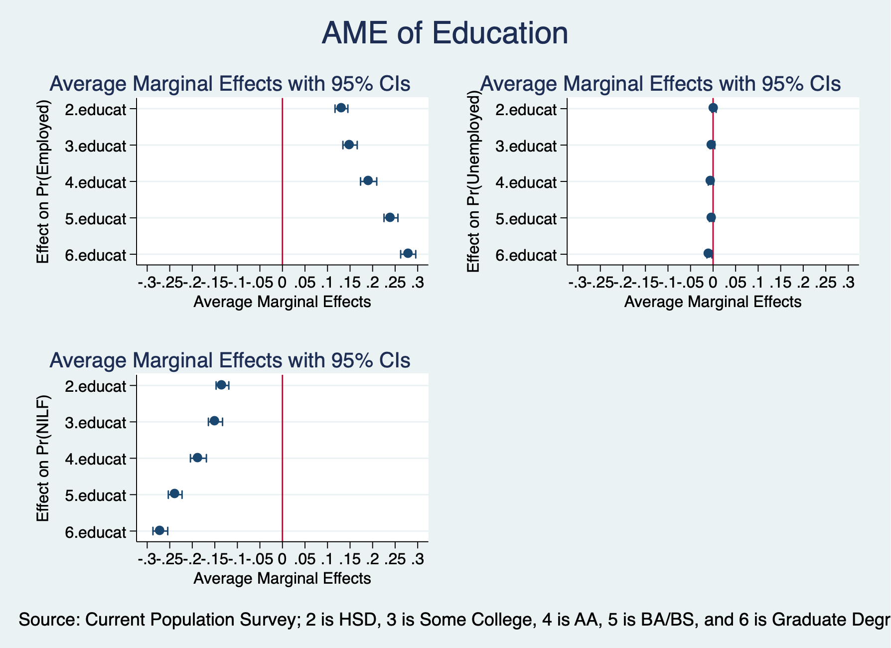
. marginsplot, allsimplelabels horizontal recast(scatter) name(Employed) yscale(reverse) ytitle("Effect on Pr(Emplo
> yed)") ///
> xtitle("Average Marginal Effects") xline(0) xlabel(-.3(.05).3)
Variables that uniquely identify margins: _deriv
Individuals with high school degree have 13.1 percentage point more likely to be employed compared to high school dropouts. Individuals with some college are 15 percentage points more likely to be employed compared to high school dropouts. Individuals with Associates or Vocational degrees are 19.1 percentage points more likely to be employed compared to high school dropouts. Individuals with a Bachelor’s degree are 24.1 percentage points more likely to be employed, while individuals with a graduate degree are 27.9 percentage points more likely to be employed compared to high school dropouts.
. margins, dydx(educat) predict(outcome(2))

Average marginal effects                        Number of obs     =     41,599
Model VCE    : OIM

Expression   : Pr(laborforcestatus==Unemployed), predict(outcome(2))
dy/dx w.r.t. : 2.educat 3.educat 4.educat 5.educat 6.educat

──────────────────────────┬────────────────────────────────────────────────────────────────
                          │            Delta-method
                          │      dy/dx   Std. Err.      z    P>|z|     [95% Conf. Interval]
──────────────────────────┼────────────────────────────────────────────────────────────────
                   educat │
                     HSD  │   .0021475   .0023962     0.90   0.370     -.002549     .006844
            Some College  │  -.0014486   .0026367    -0.55   0.583    -.0066165    .0037194
           AA/Vocational  │  -.0048071   .0030039    -1.60   0.110    -.0106946    .0010805
                   BS/BA  │  -.0028255   .0026516    -1.07   0.287    -.0080226    .0023715
Graduate or Professional  │  -.0081376   .0028311    -2.87   0.004    -.0136864   -.0025888
──────────────────────────┴────────────────────────────────────────────────────────────────
Note: dy/dx for factor levels is the discrete change from the base level.

. marginsplot, allsimplelabels horizontal recast(scatter) name(Unemployed) yscale(reverse) ytitle("Effect on Pr(Une
> mployed)") ///
> xtitle("Average Marginal Effects") xline(0) xlabel(-.3(.05).3)

  Variables that uniquely identify margins: _deriv
. margins, dydx(educat) predict(outcome(3))

Average marginal effects                        Number of obs     =     41,599
Model VCE    : OIM

Expression   : Pr(laborforcestatus==NILF), predict(outcome(3))
dy/dx w.r.t. : 2.educat 3.educat 4.educat 5.educat 6.educat

──────────────────────────┬────────────────────────────────────────────────────────────────
                          │            Delta-method
                          │      dy/dx   Std. Err.      z    P>|z|     [95% Conf. Interval]
──────────────────────────┼────────────────────────────────────────────────────────────────
                   educat │
                     HSD  │  -.1330487   .0071954   -18.49   0.000    -.1471514    -.118946
            Some College  │  -.1485456   .0079934   -18.58   0.000    -.1642124   -.1328789
           AA/Vocational  │  -.1863908   .0090294   -20.64   0.000    -.2040881   -.1686934
                   BS/BA  │  -.2379236   .0077818   -30.57   0.000    -.2531757   -.2226716
Graduate or Professional  │  -.2708111   .0083689   -32.36   0.000    -.2872139   -.2544084
──────────────────────────┴────────────────────────────────────────────────────────────────
Note: dy/dx for factor levels is the discrete change from the base level.

. marginsplot, allsimplelabels horizontal recast(scatter) name(NILF) yscale(reverse) ytitle("Effect on Pr(NILF)") /
> //
> xtitle("Average Marginal Effects") xline(0) xlabel(-.3(.05).3)

  Variables that uniquely identify margins: _deriv
Combine graphs
. graph combine Employed Unemployed NILF, ycommon title("AME of Education") ///
> note("Source: Current Population Survey; 2 is HSD, 3 is Some College, 4 is AA, 5 is BA/BS, and 6 is Graduate Degr
> ee")

. graph export "/Users/Sam/Desktop/Econ 645/Stata/week8_mnlmeducation.png", replace
(file /Users/Sam/Desktop/Econ 645/Stata/week8_mnlmeducation.png written in PNG format)
. graph drop Employed Unemployed NILF
. margins, dydx(exp) at(exp=(0(2)60)) predict(outcome(1))
Average marginal effects Number of obs = 41,599
Model VCE : OIM
Expression : Pr(laborforcestatus==Employed), predict(outcome(1))
dy/dx w.r.t. : exp
1._at : exp = 0
2._at : exp = 2
3._at : exp = 4
4._at : exp = 6
5._at : exp = 8
6._at : exp = 10
7._at : exp = 12
8._at : exp = 14
9._at : exp = 16
10._at : exp = 18
11._at : exp = 20
12._at : exp = 22
13._at : exp = 24
14._at : exp = 26
15._at : exp = 28
16._at : exp = 30
17._at : exp = 32
18._at : exp = 34
19._at : exp = 36
20._at : exp = 38
21._at : exp = 40
22._at : exp = 42
23._at : exp = 44
24._at : exp = 46
25._at : exp = 48
26._at : exp = 50
27._at : exp = 52
28._at : exp = 54
29._at : exp = 56
30._at : exp = 58
31._at : exp = 60
─────────────┬────────────────────────────────────────────────────────────────
│ Delta-method
│ dy/dx Std. Err. z P>|z| [95% Conf. Interval]
─────────────┼────────────────────────────────────────────────────────────────
exp │
_at │
1 │ .0119199 .0001127 105.73 0.000 .0116989 .0121408
2 │ .0130781 .0001155 113.28 0.000 .0128519 .0133044
3 │ .013976 .0001461 95.64 0.000 .0136896 .0142625
4 │ .0145643 .0001796 81.10 0.000 .0142123 .0149163
5 │ .0148298 .0002035 72.86 0.000 .0144308 .0152287
6 │ .0147942 .000215 68.83 0.000 .0143729 .0152155
7 │ .0145067 .0002152 67.40 0.000 .0140849 .0149285
8 │ .0140316 .0002075 67.61 0.000 .0136249 .0144384
9 │ .0134367 .0001953 68.81 0.000 .013054 .0138195
10 │ .0127838 .0001811 70.60 0.000 .0124289 .0131387
11 │ .0121231 .0001667 72.73 0.000 .0117965 .0124498
12 │ .0114913 .000153 75.12 0.000 .0111915 .0117912
13 │ .0109121 .0001403 77.76 0.000 .0106371 .0111872
14 │ .0103981 .0001289 80.69 0.000 .0101455 .0106507
15 │ .0099532 .0001186 83.95 0.000 .0097208 .0101855
16 │ .0095751 .0001094 87.52 0.000 .0093606 .0097895
17 │ .0092574 .0001014 91.30 0.000 .0090586 .0094561
18 │ .0089913 .0000945 95.12 0.000 .008806 .0091766
19 │ .0087672 .0000887 98.80 0.000 .0085933 .0089411
20 │ .0085751 .0000839 102.22 0.000 .0084107 .0087395
21 │ .0084059 .0000798 105.34 0.000 .0082495 .0085623
22 │ .0082513 .0000762 108.24 0.000 .0081019 .0084007
23 │ .0081038 .0000729 111.13 0.000 .0079609 .0082468
24 │ .0079576 .0000697 114.23 0.000 .007821 .0080941
25 │ .0078075 .0000663 117.83 0.000 .0076776 .0079373
26 │ .0076498 .0000626 122.19 0.000 .0075271 .0077725
27 │ .0074817 .0000586 127.62 0.000 .0073668 .0075967
28 │ .0073016 .0000543 134.46 0.000 .0071952 .0074081
29 │ .0071087 .0000497 143.16 0.000 .0070113 .007206
30 │ .0069031 .0000447 154.27 0.000 .0068154 .0069908
31 │ .0066862 .0000397 168.35 0.000 .0066084 .0067641
─────────────┴────────────────────────────────────────────────────────────────
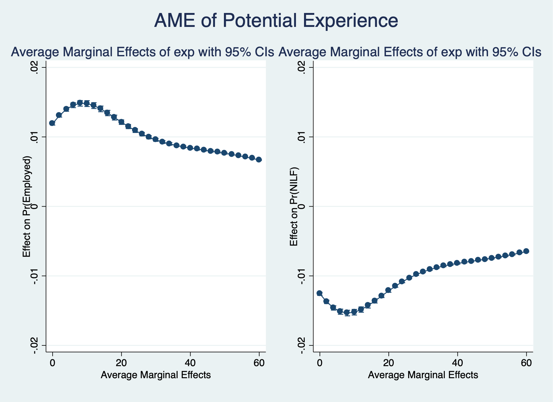
. marginsplot, allsimplelabels name(Employed) ytitle("Effect on Pr(Employed)") xtitle("Average Marginal Effects")
Variables that uniquely identify margins: exp
. margins, dydx(exp) at(exp=(0(2)60)) predict(outcome(3))

Average marginal effects                        Number of obs     =     41,599
Model VCE    : OIM

Expression   : Pr(laborforcestatus==NILF), predict(outcome(3))
dy/dx w.r.t. : exp

1._at        : exp             =           0

2._at        : exp             =           2

3._at        : exp             =           4

4._at        : exp             =           6

5._at        : exp             =           8

6._at        : exp             =          10

7._at        : exp             =          12

8._at        : exp             =          14

9._at        : exp             =          16

10._at       : exp             =          18

11._at       : exp             =          20

12._at       : exp             =          22

13._at       : exp             =          24

14._at       : exp             =          26

15._at       : exp             =          28

16._at       : exp             =          30

17._at       : exp             =          32

18._at       : exp             =          34

19._at       : exp             =          36

20._at       : exp             =          38

21._at       : exp             =          40

22._at       : exp             =          42

23._at       : exp             =          44

24._at       : exp             =          46

25._at       : exp             =          48

26._at       : exp             =          50

27._at       : exp             =          52

28._at       : exp             =          54

29._at       : exp             =          56

30._at       : exp             =          58

31._at       : exp             =          60

─────────────┬────────────────────────────────────────────────────────────────
             │            Delta-method
             │      dy/dx   Std. Err.      z    P>|z|     [95% Conf. Interval]
─────────────┼────────────────────────────────────────────────────────────────
exp          │
         _at │
          1  │  -.0125848   .0001155  -108.97   0.000    -.0128111   -.0123584
          2  │  -.0137412   .0001266  -108.55   0.000    -.0139893    -.013493
          3  │  -.0146118    .000159   -91.88   0.000    -.0149235   -.0143001
          4  │  -.0151489   .0001885   -80.35   0.000    -.0155185   -.0147794
          5  │  -.0153436   .0002048   -74.91   0.000     -.015745   -.0149421
          6  │  -.0152237   .0002061   -73.87   0.000    -.0156276   -.0148198
          7  │  -.0148454   .0001949   -76.17   0.000    -.0152274   -.0144634
          8  │  -.0142796   .0001756   -81.30   0.000    -.0146238   -.0139353
          9  │  -.0135992   .0001528   -89.00   0.000    -.0138986   -.0132997
         10  │  -.0128695   .0001299   -99.06   0.000    -.0131241   -.0126148
         11  │  -.0121426   .0001093  -111.07   0.000    -.0123569   -.0119284
         12  │  -.0114558   .0000922  -124.29   0.000    -.0116365   -.0112752
         13  │  -.0108322   .0000787  -137.62   0.000    -.0109865   -.0106779
         14  │  -.0102833   .0000686  -149.81   0.000    -.0104178   -.0101487
         15  │  -.0098117   .0000614  -159.70   0.000    -.0099321   -.0096913
         16  │  -.0094137   .0000566  -166.42   0.000    -.0095246   -.0093028
         17  │  -.0090816   .0000536  -169.49   0.000    -.0091866   -.0089766
         18  │  -.0088055   .0000521  -169.01   0.000    -.0089076   -.0087033
         19  │  -.0085745   .0000517  -165.70   0.000    -.0086759   -.0084731
         20  │   -.008378   .0000521  -160.73   0.000    -.0084802   -.0082759
         21  │  -.0082063   .0000528  -155.31   0.000    -.0083098   -.0081027
         22  │  -.0080503   .0000535  -150.38   0.000    -.0081552   -.0079453
         23  │  -.0079024   .0000539  -146.55   0.000    -.0080081   -.0077967
         24  │  -.0077563   .0000538  -144.13   0.000    -.0078617   -.0076508
         25  │  -.0076067   .0000531  -143.27   0.000    -.0077108   -.0075027
         26  │  -.0074499   .0000517  -144.07   0.000    -.0075512   -.0073485
         27  │  -.0072829   .0000497  -146.60   0.000    -.0073802   -.0071855
         28  │   -.007104    .000047  -151.07   0.000    -.0071962   -.0070118
         29  │  -.0069124   .0000438  -157.78   0.000    -.0069983   -.0068266
         30  │  -.0067085   .0000401  -167.14   0.000    -.0067872   -.0066298
         31  │  -.0064935   .0000362  -179.60   0.000    -.0065643   -.0064226
─────────────┴────────────────────────────────────────────────────────────────
Combine Graphs
. marginsplot, allsimplelabels name(NILF) ytitle("Effect on Pr(NILF)") xtitle("Average Marginal Effects")

  Variables that uniquely identify margins: exp

. graph combine Employed NILF, ycommon title("AME of Potential Experience")

. graph export "/Users/Sam/Desktop/Econ 645/Stata/week8_mnlmexp.png", replace
(file /Users/Sam/Desktop/Econ 645/Stata/week8_mnlmexp.png written in PNG format)
. graph drop Employed NILF
. est clear

. eststo mnlm: quietly mlogit laborforce i.educat exp exp2 i.race_ethnicity i.female i.metroarea i.union i.marital
Estimate the average marginal effects. Please note the post option when storing margin results
. eststo Employed: quietly margins, dydx(educat) predict(outcome(1)) post

. estimates restore mnlm
(results mnlm are active now)

. eststo Unemployed: quietly margins, dydx(educat) predict(outcome(2)) post

. estimates restore mnlm
(results mnlm are active now)

. eststo NILF: quietly margins, dydx(educat) predict(outcome(3)) post
Use coefplot
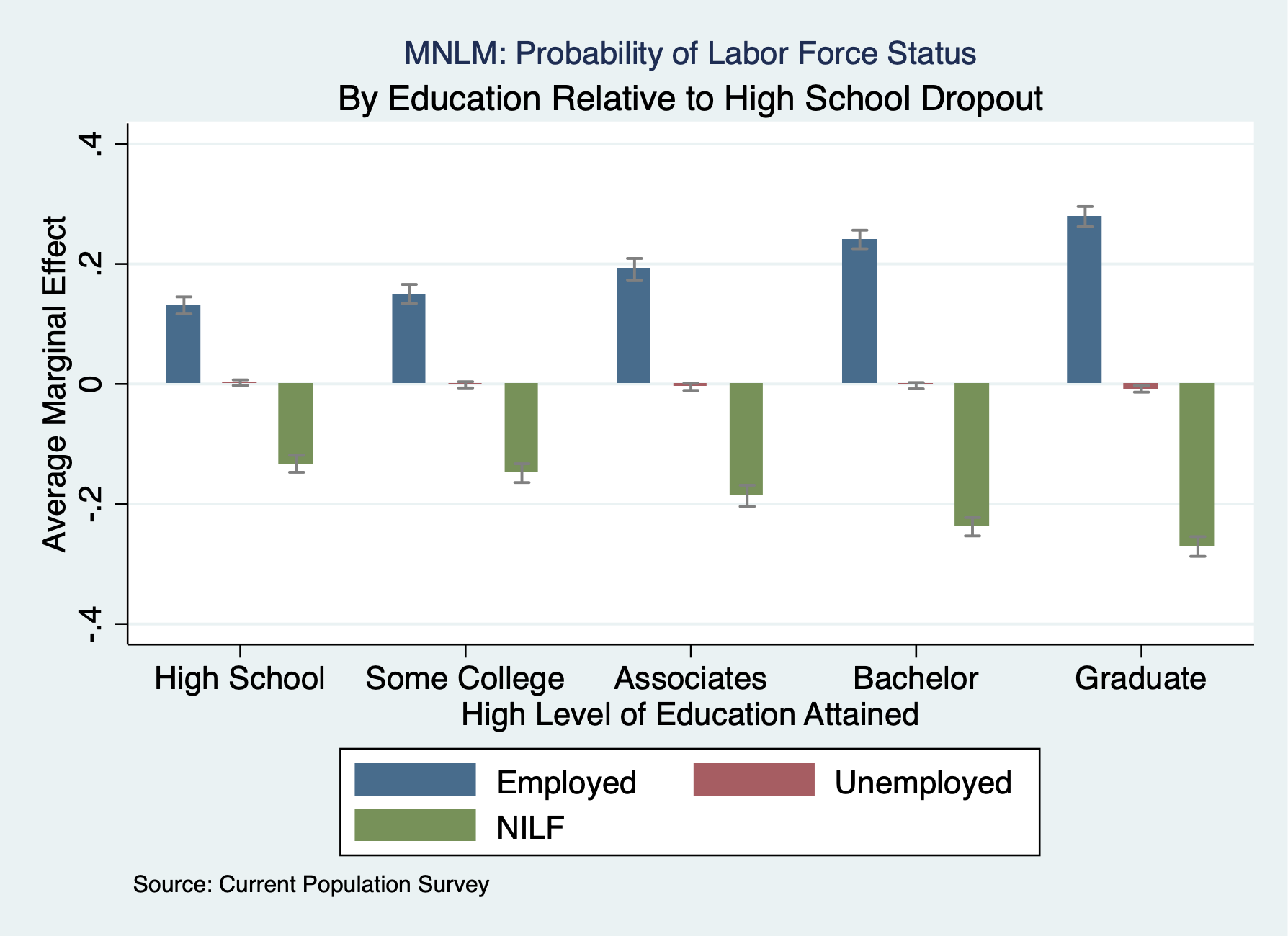
. coefplot Employed Unemployed NILF, ///
> recast(bar) barw(0.15) vertical ///
> ciopts(recast(rcap) color(gs8)) citop ///
> xlab(1 "High School" 2 "Some College" 3 "Associates" 4 "Bachelor" 5 "Graduate") ///
> ytitle("Average Marginal Effect") ///
> xtitle("High Level of Education Attained") ///
> title("MNLM: Probability of Labor Force Status", size(*0.7))    ///
> subtitle("By Education Relative to High School Dropout")    ///
> caption("Source: Current Population Survey", size(*0.75)) ///
> name(coefplot3)

. graph export "/Users/Sam/Desktop/Econ 645/Stata/week8_mnlmcoefplot.png", replace
(file /Users/Sam/Desktop/Econ 645/Stata/week8_mnlmcoefplot.png written in PNG format)
. graph drop coefplot3
We’ll look at hours of labor being supplied.
Lesson: 1) Tobit and OLS have the same sign; 2) Tobit and OLS magnitudes are not directly comparable. We need an adjustment factor, or use marginal effects.
We have data on married women’ annual labor supply with hours of work for wage in the labor force. There are 428 women employed with hours, and 325 women have no hours. Since we have a sizable about of 0 (corner soluation), we can use a Tobit model.
. use mroz.dta, clear
Summarize hours
. sum hours

    Variable │        Obs        Mean    Std. Dev.       Min        Max
─────────────┼─────────────────────────────────────────────────────────
       hours │        753    740.5764    871.3142          0       4950

. tab hours if hours == 0

      hours │      Freq.     Percent        Cum.
────────────┼───────────────────────────────────
          0 │        325      100.00      100.00
────────────┼───────────────────────────────────
      Total │        325      100.00
tab hours inlf
. tabstat hours, by(inlf) stat(mean median sd)

Summary for variables: hours
     by categories of: inlf

    inlf │      mean       p50        sd
─────────┼──────────────────────────────
       0 │         0         0         0
       1 │   1302.93    1365.5  776.2744
─────────┼──────────────────────────────
   Total │  740.5764       288  871.3142
─────────┴──────────────────────────────
We have 325 women who had 0 hours
. histogram hours
(bin=27, start=0, width=183.33333)

. graph export "/Users/Sam/Desktop/Econ 645/Stata/week8_hourhist.png", replace
(file /Users/Sam/Desktop/Econ 645/Stata/week8_hourhist.png written in PNG format)
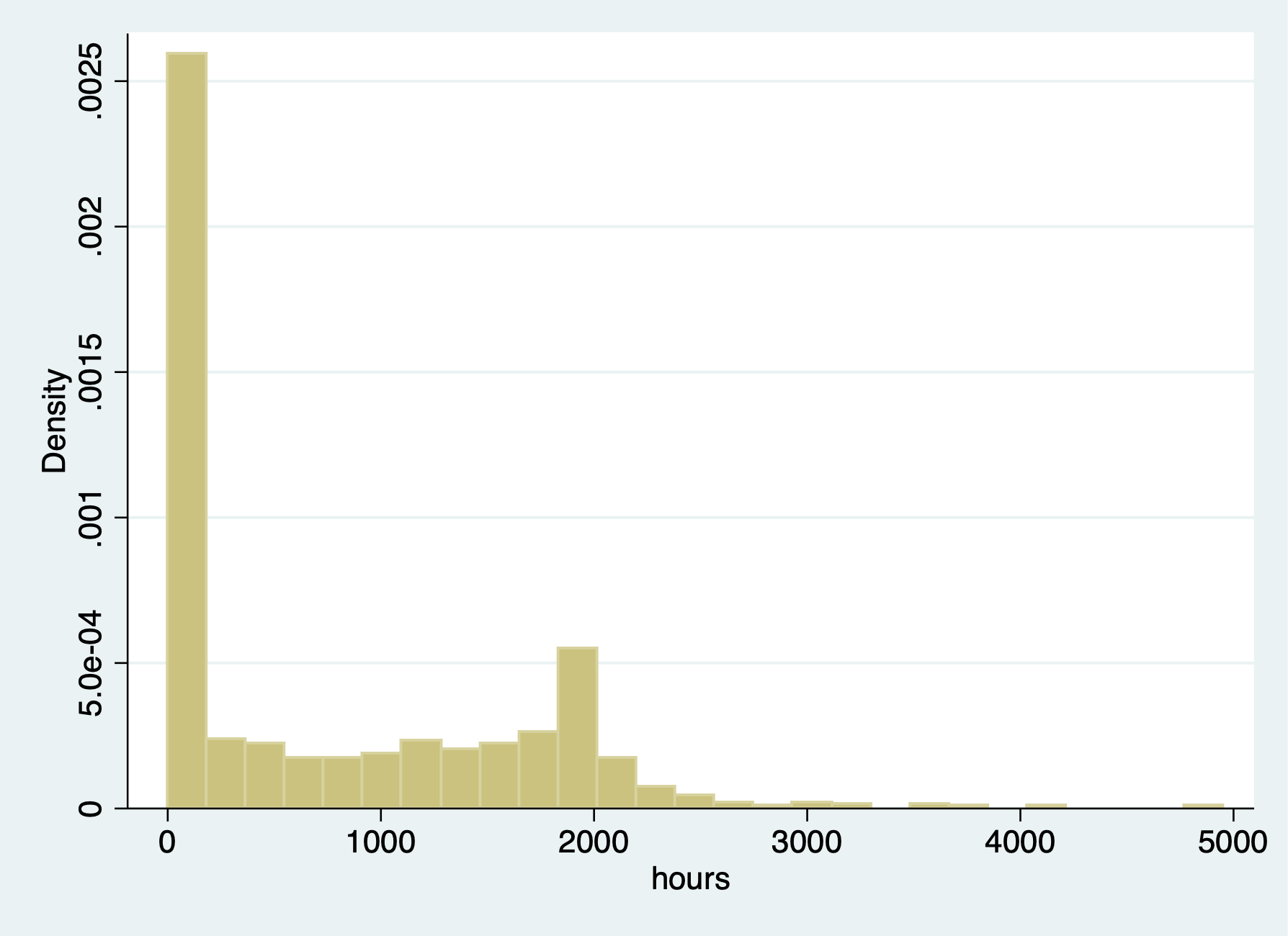 We have corner solution for
women have 0 hours of labor
We have corner solution for
women have 0 hours of labor
The range for women who do have working hours - ranges from 12 to 4950 hours
. sum hours if hours > 0

    Variable │        Obs        Mean    Std. Dev.       Min        Max
─────────────┼─────────────────────────────────────────────────────────
       hours │        428     1302.93    776.2744         12       4950
OLS Model
. est clear

. eststo OLS: reg hours nwifeinc educ exper expersq age kidslt6 kidsge6

      Source │       SS           df       MS      Number of obs   =       753
─────────────┼──────────────────────────────────   F(7, 745)       =     38.50
       Model │   151647606         7  21663943.7   Prob > F        =    0.0000
    Residual │   419262118       745  562767.944   R-squared       =    0.2656
─────────────┼──────────────────────────────────   Adj R-squared   =    0.2587
       Total │   570909724       752  759188.463   Root MSE        =    750.18

─────────────┬────────────────────────────────────────────────────────────────
       hours │      Coef.   Std. Err.      t    P>|t|     [95% Conf. Interval]
─────────────┼────────────────────────────────────────────────────────────────
    nwifeinc │  -3.446636      2.544    -1.35   0.176    -8.440898    1.547626
        educ │   28.76112   12.95459     2.22   0.027     3.329283    54.19297
       exper │   65.67251   9.962983     6.59   0.000     46.11365    85.23138
     expersq │  -.7004939   .3245501    -2.16   0.031    -1.337635   -.0633524
         age │  -30.51163   4.363868    -6.99   0.000    -39.07858   -21.94469
     kidslt6 │  -442.0899    58.8466    -7.51   0.000    -557.6148    -326.565
     kidsge6 │  -32.77923   23.17622    -1.41   0.158     -78.2777    12.71924
       _cons │   1330.482   270.7846     4.91   0.000     798.8906    1862.074
─────────────┴────────────────────────────────────────────────────────────────

. margins

Predictive margins                              Number of obs     =        753
Model VCE    : OLS

Expression   : Linear prediction, predict()

─────────────┬────────────────────────────────────────────────────────────────
             │            Delta-method
             │     Margin   Std. Err.      t    P>|t|     [95% Conf. Interval]
─────────────┼────────────────────────────────────────────────────────────────
       _cons │   740.5764   27.33803    27.09   0.000     686.9076    794.2451
─────────────┴────────────────────────────────────────────────────────────────
Tobit Model
. eststo TOBIT: tobit hours nwifeinc educ exper expersq age kidslt6 kidsge6, ll(0)

Tobit regression                                Number of obs     =        753
                                                LR chi2(7)        =     271.59
                                                Prob > chi2       =     0.0000
Log likelihood = -3819.0946                     Pseudo R2         =     0.0343

─────────────┬────────────────────────────────────────────────────────────────
       hours │      Coef.   Std. Err.      t    P>|t|     [95% Conf. Interval]
─────────────┼────────────────────────────────────────────────────────────────
    nwifeinc │  -8.814243   4.459096    -1.98   0.048    -17.56811   -.0603724
        educ │   80.64561   21.58322     3.74   0.000     38.27453    123.0167
       exper │   131.5643   17.27938     7.61   0.000     97.64231    165.4863
     expersq │  -1.864158   .5376615    -3.47   0.001    -2.919667   -.8086479
         age │  -54.40501   7.418496    -7.33   0.000    -68.96862    -39.8414
     kidslt6 │  -894.0217   111.8779    -7.99   0.000    -1113.655   -674.3887
     kidsge6 │    -16.218   38.64136    -0.42   0.675    -92.07675    59.64075
       _cons │   965.3053   446.4358     2.16   0.031     88.88528    1841.725
─────────────┼────────────────────────────────────────────────────────────────
      /sigma │   1122.022   41.57903                      1040.396    1203.647
─────────────┴────────────────────────────────────────────────────────────────
           325  left-censored observations at hours <= 0
           428     uncensored observations
             0 right-censored observations

. quietly sum exper

. local exp2=r(mean)^2
Using ystar tells Stata to act like there is no censoring even though the model allows for it Statelist Discussion 1531196
. margins, dydx(*) predict(ystar(0,.)) at(expersq=`exp2')

Average marginal effects                        Number of obs     =        753
Model VCE    : OIM

Expression   : E(hours*|hours>0), predict(ystar(0,.))
dy/dx w.r.t. : nwifeinc educ exper expersq age kidslt6 kidsge6
at           : expersq         =    113.0141

─────────────┬────────────────────────────────────────────────────────────────
             │            Delta-method
             │      dy/dx   Std. Err.      z    P>|z|     [95% Conf. Interval]
─────────────┼────────────────────────────────────────────────────────────────
    nwifeinc │  -5.223903   2.639553    -1.98   0.048    -10.39733   -.0504745
        educ │   47.79592    12.7368     3.75   0.000     22.83224     72.7596
       exper │    77.9737   9.900685     7.88   0.000     58.56872    97.37869
     expersq │  -1.104823    .316282    -3.49   0.000    -1.724724   -.4849218
         age │  -32.24401   4.348403    -7.42   0.000    -40.76672   -23.72129
     kidslt6 │  -529.8564   65.40462    -8.10   0.000    -658.0471   -401.6657
     kidsge6 │  -9.611857   22.90535    -0.42   0.675    -54.50553    35.28181
─────────────┴────────────────────────────────────────────────────────────────
. eststo AME: margins, dydx(*) predict(ystar(0,.)) at(expersq=`exp2') post

Average marginal effects                        Number of obs     =        753
Model VCE    : OIM

Expression   : E(hours*|hours>0), predict(ystar(0,.))
dy/dx w.r.t. : nwifeinc educ exper expersq age kidslt6 kidsge6
at           : expersq         =    113.0141

─────────────┬────────────────────────────────────────────────────────────────
             │            Delta-method
             │      dy/dx   Std. Err.      z    P>|z|     [95% Conf. Interval]
─────────────┼────────────────────────────────────────────────────────────────
    nwifeinc │  -5.223903   2.639553    -1.98   0.048    -10.39733   -.0504745
        educ │   47.79592    12.7368     3.75   0.000     22.83224     72.7596
       exper │    77.9737   9.900685     7.88   0.000     58.56872    97.37869
     expersq │  -1.104823    .316282    -3.49   0.000    -1.724724   -.4849218
         age │  -32.24401   4.348403    -7.42   0.000    -40.76672   -23.72129
     kidslt6 │  -529.8564   65.40462    -8.10   0.000    -658.0471   -401.6657
     kidsge6 │  -9.611857   22.90535    -0.42   0.675    -54.50553    35.28181
─────────────┴────────────────────────────────────────────────────────────────
. quietly tobit hours nwifeinc educ exper expersq age kidslt6 kidsge6, ll(0)

. eststo MEA: margins, dydx(*) predict(ystar(0,.)) at(expersq=`exp2') atmeans post

Conditional marginal effects                    Number of obs     =        753
Model VCE    : OIM

Expression   : E(hours*|hours>0), predict(ystar(0,.))
dy/dx w.r.t. : nwifeinc educ exper expersq age kidslt6 kidsge6
at           : nwifeinc        =    20.12896 (mean)
               educ            =    12.28685 (mean)
               exper           =    10.63081 (mean)
               expersq         =    113.0141
               age             =    42.53785 (mean)
               kidslt6         =    .2377158 (mean)
               kidsge6         =    1.353254 (mean)

─────────────┬────────────────────────────────────────────────────────────────
             │            Delta-method
             │      dy/dx   Std. Err.      z    P>|z|     [95% Conf. Interval]
─────────────┼────────────────────────────────────────────────────────────────
    nwifeinc │  -5.687381   2.877882    -1.98   0.048    -11.32793   -.0468358
        educ │   52.03649   13.82013     3.77   0.000     24.94954    79.12345
       exper │   84.89173   12.39757     6.85   0.000     60.59293    109.1905
     expersq │  -1.202846   .3666136    -3.28   0.001    -1.921395   -.4842964
         age │  -35.10478   4.669466    -7.52   0.000    -44.25676   -25.95279
     kidslt6 │  -576.8666   70.92986    -8.13   0.000    -715.8866   -437.8466
     kidsge6 │  -10.46465   24.93972    -0.42   0.675    -59.34561    38.41632
─────────────┴────────────────────────────────────────────────────────────────
Compare our results. Remember we cannot directly OLS and Tobit due to the scale factor.
. esttab OLS TOBIT, mtitle

────────────────────────────────────────────
                      (1)             (2)
                      OLS           TOBIT
────────────────────────────────────────────
main
nwifeinc           -3.447          -8.814*
                  (-1.35)         (-1.98)

educ                28.76*          80.65***
                   (2.22)          (3.74)

exper               65.67***        131.6***
                   (6.59)          (7.61)

expersq            -0.700*         -1.864***
                  (-2.16)         (-3.47)

age                -30.51***       -54.41***
                  (-6.99)         (-7.33)

kidslt6            -442.1***       -894.0***
                  (-7.51)         (-7.99)

kidsge6            -32.78          -16.22
                  (-1.41)         (-0.42)

_cons              1330.5***        965.3*
                   (4.91)          (2.16)
────────────────────────────────────────────
sigma
_cons                              1122.0***
                                  (26.99)
────────────────────────────────────────────
N                     753             753
────────────────────────────────────────────
t statistics in parentheses
* p<0.05, ** p<0.01, *** p<0.001
Compare OLS and Average Marginal Effects and Marginal Effects at the Average.
. esttab OLS AME MEA, mtitle("OLS" "AME" "MEA")

────────────────────────────────────────────────────────────
                      (1)             (2)             (3)
                      OLS             AME             MEA
────────────────────────────────────────────────────────────
nwifeinc           -3.447          -5.224*         -5.687*
                  (-1.35)         (-1.98)         (-1.98)

educ                28.76*          47.80***        52.04***
                   (2.22)          (3.75)          (3.77)

exper               65.67***        77.97***        84.89***
                   (6.59)          (7.88)          (6.85)

expersq            -0.700*         -1.105***       -1.203**
                  (-2.16)         (-3.49)         (-3.28)

age                -30.51***       -32.24***       -35.10***
                  (-6.99)         (-7.42)         (-7.52)

kidslt6            -442.1***       -529.9***       -576.9***
                  (-7.51)         (-8.10)         (-8.13)

kidsge6            -32.78          -9.612          -10.46
                  (-1.41)         (-0.42)         (-0.42)

_cons              1330.5***
                   (4.91)
────────────────────────────────────────────────────────────
N                     753             753             753
────────────────────────────────────────────────────────────
t statistics in parentheses
* p<0.05, ** p<0.01, *** p<0.001
When we compare marginal effects, we see that an additional year of education increases annual hours by 48 to 52 hours with the Tobit estimator. We see that an additional child less than 6 reduces the annual hours by a range of 530 to 577 hours.
Compare Graphs
. est clear
OLS Model
. quietly reg hours nwifeinc educ exper expersq age kidslt6 kidsge6

. eststo OLS: margins, at(educ=(0(2)20)) post

Predictive margins                              Number of obs     =        753
Model VCE    : OLS

Expression   : Linear prediction, predict()

1._at        : educ            =           0

2._at        : educ            =           2

3._at        : educ            =           4

4._at        : educ            =           6

5._at        : educ            =           8

6._at        : educ            =          10

7._at        : educ            =          12

8._at        : educ            =          14

9._at        : educ            =          16

10._at       : educ            =          18

11._at       : educ            =          20

─────────────┬────────────────────────────────────────────────────────────────
             │            Delta-method
             │     Margin   Std. Err.      t    P>|t|     [95% Conf. Interval]
─────────────┼────────────────────────────────────────────────────────────────
         _at │
          1  │   387.1927   161.5017     2.40   0.017        70.14    704.2453
          2  │   444.7149   136.0372     3.27   0.001     177.6531    711.7767
          3  │   502.2372    110.779     4.53   0.000      284.761    719.7133
          4  │   559.7594    85.9094     6.52   0.000     391.1061    728.4127
          5  │   617.2817   61.89861     9.97   0.000     495.7652    738.7981
          6  │   674.8039   40.31156    16.74   0.000     595.6661    753.9417
          7  │   732.3262   27.58943    26.54   0.000     678.1639    786.4884
          8  │   789.8484   35.21225    22.43   0.000     720.7214    858.9754
          9  │   847.3707    55.3281    15.32   0.000     738.7531    955.9882
         10  │   904.8929   78.89908    11.47   0.000     750.0019    1059.784
         11  │   962.4152    103.593     9.29   0.000     759.0463    1165.784
─────────────┴────────────────────────────────────────────────────────────────
Tobit Model
. quietly tobit hours nwifeinc educ exper expersq age kidslt6 kidsge6, ll(0)

. eststo Tobit: margins, at(educ=(0(2)20)) predict(e(0,6000)) post

Predictive margins                              Number of obs     =        753
Model VCE    : OIM

Expression   : E(hours|0<hours<6000), predict(e(0,6000))

1._at        : educ            =           0

2._at        : educ            =           2

3._at        : educ            =           4

4._at        : educ            =           6

5._at        : educ            =           8

6._at        : educ            =          10

7._at        : educ            =          12

8._at        : educ            =          14

9._at        : educ            =          16

10._at       : educ            =          18

11._at       : educ            =          20

─────────────┬────────────────────────────────────────────────────────────────
             │            Delta-method
             │     Margin   Std. Err.      z    P>|z|     [95% Conf. Interval]
─────────────┼────────────────────────────────────────────────────────────────
         _at │
          1  │   727.4644   76.74259     9.48   0.000     577.0517    877.8772
          2  │   773.4964   71.05237    10.89   0.000     634.2364    912.7565
          3  │   823.5401   63.95927    12.88   0.000     698.1822    948.8979
          4  │   877.8933   55.47809    15.82   0.000     769.1582    986.6283
          5  │   936.8485   45.95104    20.39   0.000     846.7861    1026.911
          6  │   1000.685   36.67591    27.28   0.000     928.8013    1072.568
          7  │   1069.659   31.51807    33.94   0.000     1007.885    1131.433
          8  │   1143.997   36.60999    31.25   0.000     1072.242    1215.751
          9  │   1223.883   52.37388    23.37   0.000     1121.232    1326.534
         10  │   1309.452   75.03347    17.45   0.000      1162.39    1456.515
         11  │   1400.783   102.4283    13.68   0.000     1200.027    1601.539
─────────────┴────────────────────────────────────────────────────────────────
. coefplot (OLS, ciopts(recast(rline) lpattern(solid))) ///
> (Tobit, ciopts(recast(rline) lpattern(dash))), at recast(line)

. graph export "/Users/Sam/Desktop/Econ 645/Stata/week8_tobitols.png", replace
(file /Users/Sam/Desktop/Econ 645/Stata/week8_tobitols.png written in PNG format)
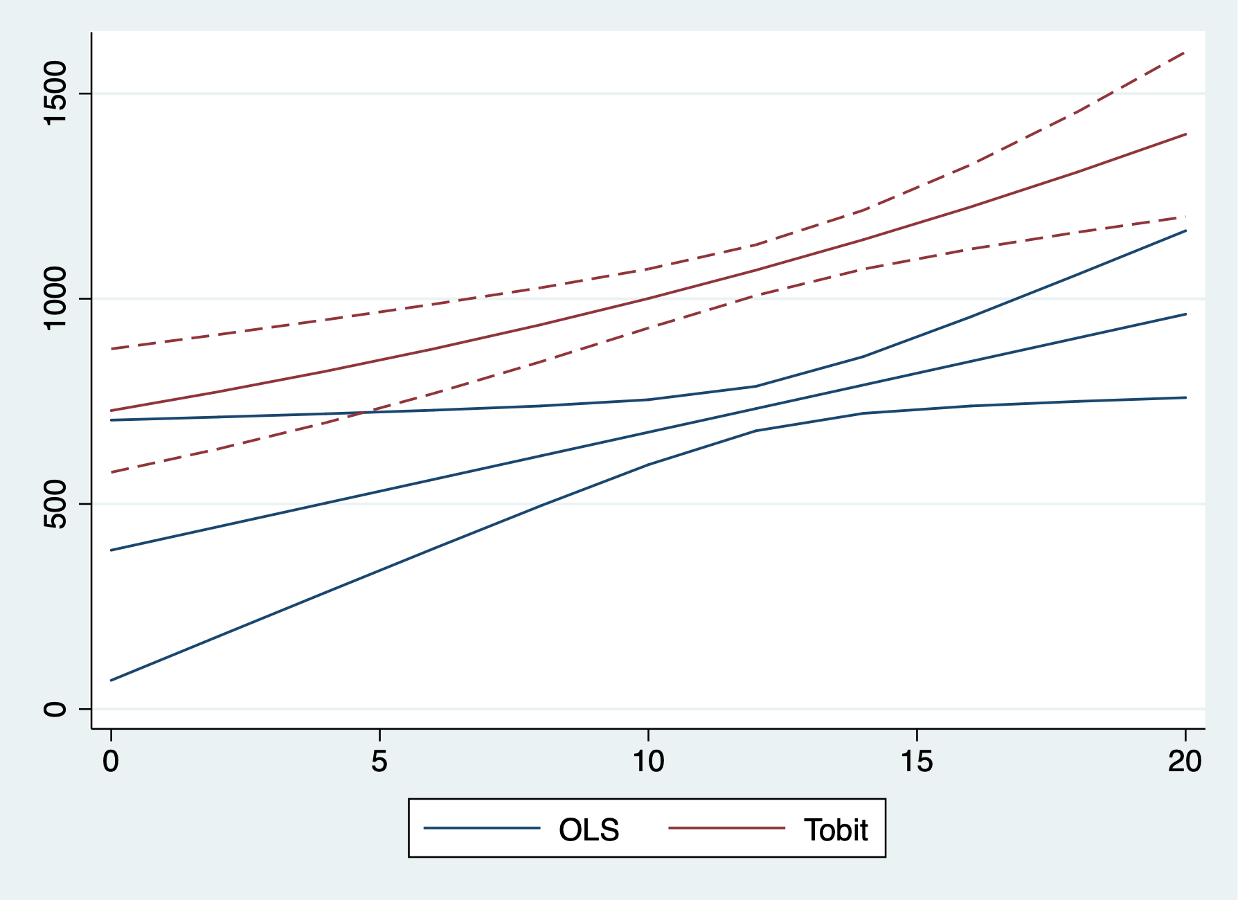
Set Working Directory
. cd "/Users/Sam/Desktop/Econ 645/Data/Mitchell"
/Users/Sam/Desktop/Econ 645/Data/Mitchell
One thing Stata easily provides are commands and options for subgroup analysis. We can use the by prefix command to create and analyze subgroups or cross-sectional units in a panel data set.
Tabulate is a very helpful command to analyze categorical variables, or occassionally look through continuous variables (as long as there aren’t too many values). The tabulate command has an option to summarize a continuous variable when tabulating categorical variables.
. use wws2, clear
(Working Women Survey w/fixes)

. tabulate married, summarize(wage)

            │       Summary of hourly wage
    married │        Mean   Std. Dev.       Freq.
────────────┼────────────────────────────────────
          0 │   8.0920006    6.354849         804
          1 │   7.6319496   5.5017864       1,440
────────────┼────────────────────────────────────
      Total │   7.7967807   5.8245895       2,244
Another option is using the bysort prefix command
. bysort married: summarize wage

───────────────────────────────────────────────────────────────────────────────────────────────────────────────────
-> married = 0

    Variable │        Obs        Mean    Std. Dev.       Min        Max
─────────────┼─────────────────────────────────────────────────────────
        wage │        804    8.092001    6.354849          0   40.19808

───────────────────────────────────────────────────────────────────────────────────────────────────────────────────
-> married = 1

    Variable │        Obs        Mean    Std. Dev.       Min        Max
─────────────┼─────────────────────────────────────────────────────────
        wage │      1,440     7.63195    5.501786   1.004952   40.74659
We can also correlate data within groups instead of using qualifiers and additional statements With qualifiers
. correlate wage age if married == 0
(obs=804)

             │     wage      age
─────────────┼──────────────────
        wage │   1.0000
         age │  -0.0185   1.0000


. correlate wage age if married == 1
(obs=1,440)

             │     wage      age
─────────────┼──────────────────
        wage │   1.0000
         age │   0.0049   1.0000
Using bysort accomplishes this in one command
. bysort married: correlate wage age

───────────────────────────────────────────────────────────────────────────────────────────────────────────────────
-> married = 0
(obs=804)

             │     wage      age
─────────────┼──────────────────
        wage │   1.0000
         age │  -0.0185   1.0000


───────────────────────────────────────────────────────────────────────────────────────────────────────────────────
-> married = 1
(obs=1,440)

             │     wage      age
─────────────┼──────────────────
        wage │   1.0000
         age │   0.0049   1.0000
Using bysort accomplishes even faster if we have a categorical variable with many categories
. bysort race: correlate wage age

───────────────────────────────────────────────────────────────────────────────────────────────────────────────────
-> race = 1
(obs=1,637)

             │     wage      age
─────────────┼──────────────────
        wage │   1.0000
         age │   0.0017   1.0000


───────────────────────────────────────────────────────────────────────────────────────────────────────────────────
-> race = 2
(obs=581)

             │     wage      age
─────────────┼──────────────────
        wage │   1.0000
         age │  -0.0331   1.0000


───────────────────────────────────────────────────────────────────────────────────────────────────────────────────
-> race = 3
(obs=26)

             │     wage      age
─────────────┼──────────────────
        wage │   1.0000
         age │  -0.2194   1.0000
The by prefix command and the egen command is a powerful combination that makes aggregating group statistics much easier than other statistical software packages Bysort and egen makes aggregating by groups much easier than other software. R has aggregate which is flexible and powerful, but requires more coding.
I’m not the biggest fan of Mitchell’s examples with bysort var: egen, but they get the job done. I would like us to use some CPS examples with bysort and egen.
With bysort var: egen we can calculate subgroup statistics, counts, summations with one easy line of code
. use tv1, clear

. list, sepby(kidid)

     ┌────────────────────────────────────────────┐
     │ kidid          dt   female   wt   tv   vac │
     ├────────────────────────────────────────────┤
  1. │     1   07jan2002        1   53    1     1 │
  2. │     1   08jan2002        1   55    3     1 │
     ├────────────────────────────────────────────┤
  3. │     2   16jan2002        1   58    8     1 │
     ├────────────────────────────────────────────┤
  4. │     3   18jan2002        0   60    2     0 │
  5. │     3   19jan2002        0   63    5     1 │
  6. │     3   21jan2002        0   66    1     1 │
  7. │     3   22jan2002        0   64    6     0 │
     ├────────────────────────────────────────────┤
  8. │     4   10jan2002        1   62    7     0 │
  9. │     4   11jan2002        1   58    1     0 │
 10. │     4   13jan2002        1   55    4     0 │
     └────────────────────────────────────────────┘
If we want to calculate the average tv time for each kid we first sort by the child id and then use egen. We may have multiple levels and we can use bysort to find the multiple level identifiers such as id, year, and month of year
. bysort kidid: egen avgtv = mean(tv)

. sort kidid

. list kidid tv avgtv, sepby(kidid)

     ┌────────────────────┐
     │ kidid   tv   avgtv │
     ├────────────────────┤
  1. │     1    1       2 │
  2. │     1    3       2 │
     ├────────────────────┤
  3. │     2    8       8 │
     ├────────────────────┤
  4. │     3    2     3.5 │
  5. │     3    5     3.5 │
  6. │     3    1     3.5 │
  7. │     3    6     3.5 │
     ├────────────────────┤
  8. │     4    7       4 │
  9. │     4    1       4 │
 10. │     4    4       4 │
     └────────────────────┘
If we want the standard deviation of the child’s tv watching
. bysort kidid: egen sdtv = sd(tv)
(1 missing value generated)
Let’s generate some z-scores
. generate ztv = (tv-avgtv)/sdtv
(1 missing value generated)
Let’s look at our statistics
. list

     ┌─────────────────────────────────────────────────────────────────────────────┐
     │ kidid          dt   female   wt   tv   vac   avgtv        sdtv          ztv │
     ├─────────────────────────────────────────────────────────────────────────────┤
  1. │     1   07jan2002        1   53    1     1       2   1.4142136   -.70710678 │
  2. │     1   08jan2002        1   55    3     1       2   1.4142136    .70710678 │
  3. │     2   16jan2002        1   58    8     1       8           .            . │
  4. │     3   18jan2002        0   60    2     0     3.5   2.3804761   -.63012604 │
  5. │     3   19jan2002        0   63    5     1     3.5   2.3804761    .63012604 │
     ├─────────────────────────────────────────────────────────────────────────────┤
  6. │     3   21jan2002        0   66    1     1     3.5   2.3804761   -1.0502101 │
  7. │     3   22jan2002        0   64    6     0     3.5   2.3804761    1.0502101 │
  8. │     4   10jan2002        1   62    7     0       4           3            1 │
  9. │     4   11jan2002        1   58    1     0       4           3           -1 │
 10. │     4   13jan2002        1   55    4     0       4           3            0 │
     └─────────────────────────────────────────────────────────────────────────────┘
Let’s generate some subgroup statistics for a binary variable vac Where vac=0 if the kid was not on vacation and vac=1 if the kid was on vacation
. bysort kidid: egen vac_total = total(vac)

. bysort kidid: egen vac_sd = sd(vac)
(1 missing value generated)

. bysort kidid: egen vac_min = min(vac)

. bysort kidid: egen vac_max = max(vac)

. list kidid vac*, sepby(kidid) abb(10)

     ┌─────────────────────────────────────────────────────────┐
     │ kidid   vac   vac_total      vac_sd   vac_min   vac_max │
     ├─────────────────────────────────────────────────────────┤
  1. │     1     1           2           0         1         1 │
  2. │     1     1           2           0         1         1 │
     ├─────────────────────────────────────────────────────────┤
  3. │     2     1           1           .         1         1 │
     ├─────────────────────────────────────────────────────────┤
  4. │     3     0           2   .57735027         0         1 │
  5. │     3     1           2   .57735027         0         1 │
  6. │     3     1           2   .57735027         0         1 │
  7. │     3     0           2   .57735027         0         1 │
     ├─────────────────────────────────────────────────────────┤
  8. │     4     0           0           0         0         0 │
  9. │     4     0           0           0         0         0 │
 10. │     4     0           0           0         0         0 │
     └─────────────────────────────────────────────────────────┘
Let’s see if some kids watch less than 4 hours of tv per day. We’ll generate a binary/dummy variable to be 1 if equal to or less than 4 hours a day and 0 if it is greater than 4 hours a day.
. generate tvlo = (tv < 4) if !missing(tv)
We can generate individual level subgroup analysis with bysort and egen on binary variables
. bysort kidid: egen tvlocnt = count(tvlo)

. bysort kidid: egen tvlototal = total(tvlo)

. bysort kidid: egen tvlosum = sum(tvlo)

. bysort kidid: gen tvlosum2 = sum(tvlo)

. bysort kidid: egen tvlosame = sd(tvlo)
(1 missing value generated)

. bysort kidid: egen tvloall = min(tvlo)

. bysort kidid: egen tvloever = max(tvlo)

. list kidid tv tvlo*, sepby(kidid) abb(20)

     ┌───────────────────────────────────────────────────────────────────────────────────────────────┐
     │ kidid   tv   tvlo   tvlocnt   tvlototal   tvlosum   tvlosum2    tvlosame   tvloall   tvloever │
     ├───────────────────────────────────────────────────────────────────────────────────────────────┤
  1. │     1    1      1         2           2         2          1           0         1          1 │
  2. │     1    3      1         2           2         2          2           0         1          1 │
     ├───────────────────────────────────────────────────────────────────────────────────────────────┤
  3. │     2    8      0         1           0         0          0           .         0          0 │
     ├───────────────────────────────────────────────────────────────────────────────────────────────┤
  4. │     3    2      1         4           2         2          1   .57735027         0          1 │
  5. │     3    5      0         4           2         2          1   .57735027         0          1 │
  6. │     3    1      1         4           2         2          2   .57735027         0          1 │
  7. │     3    6      0         4           2         2          2   .57735027         0          1 │
     ├───────────────────────────────────────────────────────────────────────────────────────────────┤
  8. │     4    7      0         3           1         1          0   .57735027         0          1 │
  9. │     4    1      1         3           1         1          1   .57735027         0          1 │
 10. │     4    4      0         3           1         1          1   .57735027         0          1 │
     └───────────────────────────────────────────────────────────────────────────────────────────────┘
Notice how count() provides the number of observations for each kid, while total() returns a constant for the sum of all values, but so does egen sum(). The problem is that there is a gen var = sum(var2) function that returns a running sum that we see in tvsum2. I usually use egen sum, but I think egen total() is the more appropriate function to use when returning a constant.
We have our central tendencies functions with mean(), median(), and mode(). We can find percentiles with pctile(var), p(#). We have other egen functions that may be of help, such as iqr(), Median Absolute Deviation mad(), Mean Absolute Deviation mdev(), kurt(), skew(), etc.
. help egen
Mitchell has a good note here Egen mean() takes an arguement, not a varlist, so if you put bysort idvar: egen meanvars1_5=mean(var1-var5), mean() will return not the means of vars 1 through 5, but var1 minus var5
Unsolicated Opinion Alert: Subscripting (or I may accidently call it indexing) is a very powerful tool that I personally think puts Stata as the top paid statistical software (I do think that R is more powerful and more flexible, but Stata balances power, flexibility, and ease of learning).
. use tv1, clear
Each variable is a vector x1=x[x11, x12, x13,…,x1N] for i=1,…,N observations We can use a subscript or index to call which part of the vector we want to return.
. list, sepby(kidid)

     ┌────────────────────────────────────────────┐
     │ kidid          dt   female   wt   tv   vac │
     ├────────────────────────────────────────────┤
  1. │     1   07jan2002        1   53    1     1 │
  2. │     1   08jan2002        1   55    3     1 │
     ├────────────────────────────────────────────┤
  3. │     2   16jan2002        1   58    8     1 │
     ├────────────────────────────────────────────┤
  4. │     3   18jan2002        0   60    2     0 │
  5. │     3   19jan2002        0   63    5     1 │
  6. │     3   21jan2002        0   66    1     1 │
  7. │     3   22jan2002        0   64    6     0 │
     ├────────────────────────────────────────────┤
  8. │     4   10jan2002        1   62    7     0 │
  9. │     4   11jan2002        1   58    1     0 │
 10. │     4   13jan2002        1   55    4     0 │
     └────────────────────────────────────────────┘
If we want the first observation in our tv vector we can call it with [1]
. display tv[1]
1
We can look at the first kid id and date and time
. display "kid: " kidid[1] ", Date: " dt[1] ", Sex: " female[1] ", TV Hours: " tv[1]
kid: 1, Date: 15347, Sex: 1, TV Hours: 1
We can see the second observation
. display tv[2]
3
We can see the difference between the two observations
. display tv[2]-tv[1]
2
Note: we have some very useful system variables of _N and _n _N is total number of observations and when used in the subscript/index it will return the last observation
_n is current number of observations or observation number and when used in the subscript/index it will return the current observation (almost like i=i+1)
. help system variables
Subscripting is very helpful when working Panel Data. You can index within cross-sectional units over time with ease. The subscript (or index) will return the nth observation given
. use tv1, clear
If we want the first observation to be compared to all observations
. bysort kidid: gen tv_1ob = tv[1]

. list kidid tv tv_1ob, sepby(kidid)

     ┌─────────────────────┐
     │ kidid   tv   tv_1ob │
     ├─────────────────────┤
  1. │     1    1        1 │
  2. │     1    3        1 │
     ├─────────────────────┤
  3. │     2    8        8 │
     ├─────────────────────┤
  4. │     3    2        2 │
  5. │     3    5        2 │
  6. │     3    1        2 │
  7. │     3    6        2 │
     ├─────────────────────┤
  8. │     4    7        7 │
  9. │     4    1        7 │
 10. │     4    4        7 │
     └─────────────────────┘
If we want to compare the last observation to all observations
. bysort kidid: gen tv_lastob = tv[_N]

. list kidid tv tv_lastob, sepby(kidid)

     ┌───────────────────────┐
     │ kidid   tv   tv_las~b │
     ├───────────────────────┤
  1. │     1    1          3 │
  2. │     1    3          3 │
     ├───────────────────────┤
  3. │     2    8          8 │
     ├───────────────────────┤
  4. │     3    2          6 │
  5. │     3    5          6 │
  6. │     3    1          6 │
  7. │     3    6          6 │
     ├───────────────────────┤
  8. │     4    7          4 │
  9. │     4    1          4 │
 10. │     4    4          4 │
     └───────────────────────┘
If we want the second to last observation
. bysort kidid: gen tv_2tolastob = tv[_N-1]
(1 missing value generated)

. list kidid tv tv_2tolastob, sepby(kidid)

     ┌───────────────────────┐
     │ kidid   tv   tv_2to~b │
     ├───────────────────────┤
  1. │     1    1          1 │
  2. │     1    3          1 │
     ├───────────────────────┤
  3. │     2    8          . │
     ├───────────────────────┤
  4. │     3    2          1 │
  5. │     3    5          1 │
  6. │     3    1          1 │
  7. │     3    6          1 │
     ├───────────────────────┤
  8. │     4    7          1 │
  9. │     4    1          1 │
 10. │     4    4          1 │
     └───────────────────────┘
If we want the prior observation (lag of 1)
. bysort kidid: gen tv_lagob = tv[_n-1]
(4 missing values generated)

. list kidid tv tv_lagob, sepby(kidid)

     ┌───────────────────────┐
     │ kidid   tv   tv_lagob │
     ├───────────────────────┤
  1. │     1    1          . │
  2. │     1    3          1 │
     ├───────────────────────┤
  3. │     2    8          . │
     ├───────────────────────┤
  4. │     3    2          . │
  5. │     3    5          2 │
  6. │     3    1          5 │
  7. │     3    6          1 │
     ├───────────────────────┤
  8. │     4    7          . │
  9. │     4    1          7 │
 10. │     4    4          1 │
     └───────────────────────┘
If we want the next observation (lead of 1)
. bysort kidid: gen tv_leadob = tv[_n+1]
(4 missing values generated)

. list kidid tv tv_leadob, sepby(kidid)

     ┌───────────────────────┐
     │ kidid   tv   tv_lea~b │
     ├───────────────────────┤
  1. │     1    1          3 │
  2. │     1    3          . │
     ├───────────────────────┤
  3. │     2    8          . │
     ├───────────────────────┤
  4. │     3    2          5 │
  5. │     3    5          1 │
  6. │     3    1          6 │
  7. │     3    6          . │
     ├───────────────────────┤
  8. │     4    7          1 │
  9. │     4    1          4 │
 10. │     4    4          . │
     └───────────────────────┘
You can use bysort kidid (dt) to tell Stata to order by kid id and date, but NOT INCLUDE dt in the grouping. If we use kidid AND tv bysort kidid tv: egen, then we will look for observation Within kid id AND the date. Since there is only 1 observation per kid per date, we will only have 1 observation for each grouping.
. use tv1, clear
If we want the first observation to be compared to all observations
. bysort kidid (dt): gen tv_1ob1 = tv[1]

. bysort kidid dt: gen tv_1ob2 = tv[1]
Compare
. list kidid tv tv_1ob*, sepby(kidid)

     ┌────────────────────────────────┐
     │ kidid   tv   tv_1ob1   tv_1ob2 │
     ├────────────────────────────────┤
  1. │     1    1         1         1 │
  2. │     1    3         1         3 │
     ├────────────────────────────────┤
  3. │     2    8         8         8 │
     ├────────────────────────────────┤
  4. │     3    2         2         2 │
  5. │     3    5         2         5 │
  6. │     3    1         2         1 │
  7. │     3    6         2         6 │
     ├────────────────────────────────┤
  8. │     4    7         7         7 │
  9. │     4    1         7         1 │
 10. │     4    4         7         4 │
     └────────────────────────────────┘
If we want to compare the last observation to all observations
. bysort kidid (dt): gen tv_lastob1 = tv[_N]

. bysort kidid dt: gen tv_lastob2 = tv[_N]
Compare
. list kidid tv tv_lastob*, sepby(kidid)

     ┌──────────────────────────────────┐
     │ kidid   tv   tv_las~1   tv_las~2 │
     ├──────────────────────────────────┤
  1. │     1    1          3          1 │
  2. │     1    3          3          3 │
     ├──────────────────────────────────┤
  3. │     2    8          8          8 │
     ├──────────────────────────────────┤
  4. │     3    2          6          2 │
  5. │     3    5          6          5 │
  6. │     3    1          6          1 │
  7. │     3    6          6          6 │
     ├──────────────────────────────────┤
  8. │     4    7          4          7 │
  9. │     4    1          4          1 │
 10. │     4    4          4          4 │
     └──────────────────────────────────┘
If we want the prior observation (lag of 1)
. bysort kidid (dt): gen tv_lagob1 = tv[_n-1]
(4 missing values generated)

. bysort kidid dt: gen tv_lagob2 = tv[_n-1]
(10 missing values generated)
Compare
. list kidid tv tv_lagob*, sepby(kidid)

     ┌──────────────────────────────────┐
     │ kidid   tv   tv_lag~1   tv_lag~2 │
     ├──────────────────────────────────┤
  1. │     1    1          .          . │
  2. │     1    3          1          . │
     ├──────────────────────────────────┤
  3. │     2    8          .          . │
     ├──────────────────────────────────┤
  4. │     3    2          .          . │
  5. │     3    5          2          . │
  6. │     3    1          5          . │
  7. │     3    6          1          . │
     ├──────────────────────────────────┤
  8. │     4    7          .          . │
  9. │     4    1          7          . │
 10. │     4    4          1          . │
     └──────────────────────────────────┘
Another powerful combination with subscripting/indexing is that we can the generate command to create new variables that perform mathematical operators on different observations WITHIN the vector
. use tv1, clear
Difference in tv time between current period and prior period
. bysort kidid (dt): generate tvdfp = tv - tv[_n-1]
(4 missing values generated)
Difference in tv time between current period and next period
. bysort kidid (dt): generate tvdfs = tv - tv[_n+1]
(4 missing values generated)
Difference in tv time between current period and first period
. bysort kidid (dt): generate tvdff = tv - tv[1]
Difference in tv time between current period and last period
. bysort kidid (dt): generate tvdfl = tv - tv[_N]
Difference between current period and 3-year moving average over time
. bysort kidid (dt): generate tv3avg = (tv[_n-1] + tv[_n] + tv[_n+1])/3
(7 missing values generated)
. list kidid dt tvd* tv3avg

     ┌───────────────────────────────────────────────────────────────┐
     │ kidid          dt   tvdfp   tvdfs   tvdff   tvdfl      tv3avg │
     ├───────────────────────────────────────────────────────────────┤
  1. │     1   07jan2002       .      -2       0      -2           . │
  2. │     1   08jan2002       2       .       2       0           . │
  3. │     2   16jan2002       .       .       0       0           . │
  4. │     3   18jan2002       .      -3       0      -4           . │
  5. │     3   19jan2002       3       4       3      -1   2.6666667 │
     ├───────────────────────────────────────────────────────────────┤
  6. │     3   21jan2002      -4      -5      -1      -5           4 │
  7. │     3   22jan2002       5       .       4       0           . │
  8. │     4   10jan2002       .       6       0       3           . │
  9. │     4   11jan2002      -6      -3      -6      -3           4 │
 10. │     4   13jan2002       3       .      -3       0           . │
     └───────────────────────────────────────────────────────────────┘
We can also rebase our vector. For example, we can rebase a deflator for the period dollars we want.
. import excel using "cpi_1993_2023.xlsx", cellrange(A12:P42) firstrow clear

. keep Year Annual
Rebase in 1993 Dollars
. gen rebase93 = Annual/Annual[1]*100
Rebase in 2022 Dollars
. gen rebase22 = Annual/Annual[_N]*100
Rebase to 2012
. gen rebase12 = Annual/Annual[_N-10]*100

. list

     ┌────────────────────────────────────────────────────┐
     │ Year    Annual    rebase93    rebase22    rebase12 │
     ├────────────────────────────────────────────────────┤
  1. │ 1993     144.5         100   49.375545   62.937185 │
  2. │ 1994     148.2   102.56055   50.639832   64.548725 │
  3. │ 1995     152.4   105.46713   52.074969   66.378041 │
  4. │ 1996     156.9   108.58131   53.612616   68.338023 │
  5. │ 1997     160.5   111.07266   54.842733   69.906008 │
     ├────────────────────────────────────────────────────┤
  6. │ 1998       163   112.80277   55.696981   70.994887 │
  7. │ 1999     166.6   115.29412   56.927098   72.562872 │
  8. │ 2000     172.2   119.16955   58.840614    75.00196 │
  9. │ 2001     177.1   122.56055   60.514941   77.136162 │
 10. │ 2002     179.9   124.49827   61.471699   78.355706 │
     ├────────────────────────────────────────────────────┤
 11. │ 2003       184   127.33564   62.872666   80.141467 │
 12. │ 2004     188.9   130.72664   64.546992   82.275669 │
 13. │ 2005     195.3   135.15571   66.733868   85.063199 │
 14. │ 2006     201.6   139.51557   68.886573   87.807173 │
 15. │ 2007   207.342   143.48927    70.84861   90.308109 │
     ├────────────────────────────────────────────────────┤
 16. │ 2008   215.303   148.99862   73.568878   93.775534 │
 17. │ 2009   214.537   148.46851   73.307136   93.441902 │
 18. │ 2010   218.056   150.90381   74.509576   94.974607 │
 19. │ 2011   224.939   155.66713   76.861492   97.972508 │
 20. │ 2012   229.594   158.88858   78.452102         100 │
     ├────────────────────────────────────────────────────┤
 21. │ 2013   232.957   161.21592   79.601237   101.46476 │
 22. │ 2014   236.736   163.83114   80.892518   103.11071 │
 23. │ 2015   237.017   164.02561   80.988536    103.2331 │
 24. │ 2016   240.007   166.09481   82.010217    104.5354 │
 25. │ 2017    245.12   169.63322   83.757325   106.76237 │
     ├────────────────────────────────────────────────────┤
 26. │ 2018   251.107   173.77647   85.803079   109.37002 │
 27. │ 2019   255.657   176.92526    87.35781   111.35178 │
 28. │ 2020   258.811   179.10796    88.43553   112.72551 │
 29. │ 2021    270.97   187.52249   92.590251   118.02138 │
 30. │ 2022   292.655   202.52941         100   127.46631 │
     └────────────────────────────────────────────────────┘
. graph twoway line Annual Year || line rebase93 Year || ///
> line rebase22 Year, yline(100) ///
> legend(order(1 "100=1982" 2 "100=1993" 3 "100=2022"))

. graph export "/Users/Sam/Desktop/Econ 645/Stata/week8_bls.png", replace
(file /Users/Sam/Desktop/Econ 645/Stata/week8_bls.png written in PNG format)
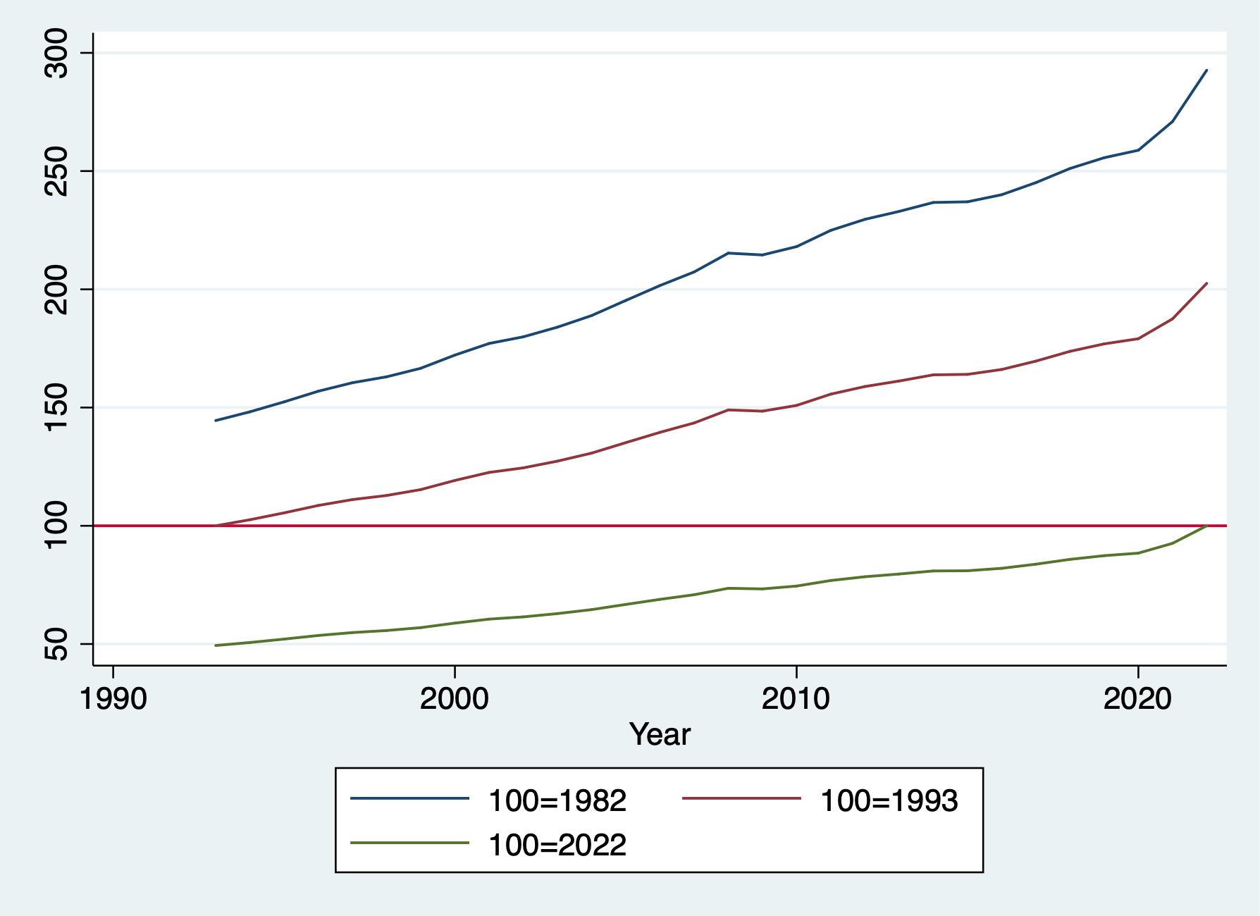
As we mentioned earlier, when we use egen sum vs gen sum, we get different results. Egen sum() is similar to egen total() but it can be confusing. When we use gen with sum(), we generate a RUNNING sum not a constant of total.
. use tv1, clear
We can generate the tv running sum across all individuals over time
. generate tvrunsum = sum(tv)
We can generate the tv running sum within an individuals time period
. bysort kidid (dt): generate bytvrunsum=sum(tv)
We can generate the total sum with an individuals time period
. bysort kidid (dt): egen bytvsum=total(tv)
We can generate the total sum for all individuals over time
. egen tvsum = total(tv)
We can also calculate a running average
. bysort kidid (dt): generate bytvrunavg=sum(tv)/_n
We can compute the individual’s average average
. bysort kidid (dt): egen bytvavg = mean(tv)
. list kidid tv tv* by*, sepby(kidid)

     ┌───────────────────────────────────────────────────────────────────────────────┐
     │ kidid   tv   tv   tvrunsum   tvsum   bytvru~m   bytvsum   bytvrun~g   bytvavg │
     ├───────────────────────────────────────────────────────────────────────────────┤
  1. │     1    1    1          1      38          1         4           1         2 │
  2. │     1    3    3          4      38          4         4           2         2 │
     ├───────────────────────────────────────────────────────────────────────────────┤
  3. │     2    8    8         12      38          8         8           8         8 │
     ├───────────────────────────────────────────────────────────────────────────────┤
  4. │     3    2    2         14      38          2        14           2       3.5 │
  5. │     3    5    5         19      38          7        14         3.5       3.5 │
  6. │     3    1    1         20      38          8        14   2.6666667       3.5 │
  7. │     3    6    6         26      38         14        14         3.5       3.5 │
     ├───────────────────────────────────────────────────────────────────────────────┤
  8. │     4    7    7         33      38          7        12           7         4 │
  9. │     4    1    1         34      38          8        12           4         4 │
 10. │     4    4    4         38      38         12        12           4         4 │
     └───────────────────────────────────────────────────────────────────────────────┘
There are other useful calculations we can do with subscripting/indexing. Some do overlap with egen, but it is helpful to know the differences.
Count the number of observations: this can be done with subscripting or egen depending upon what we want
. use tv1, clear
Generate total observation count per individual missing or not missing:
. bysort kidid (dt): generate idcount=_N
Generate the total observation without missing
. bysort kidid (dt): egen idcount_nomiss = count(tv)
Generate a running count of an observation
. bysort kidid (dt): gen idruncount = _n

. list, sepby(kidid)

     ┌────────────────────────────────────────────────────────────────────────────┐
     │ kidid          dt   female   wt   tv   vac   idcount   idcoun~s   idrunc~t │
     ├────────────────────────────────────────────────────────────────────────────┤
  1. │     1   07jan2002        1   53    1     1         2          2          1 │
  2. │     1   08jan2002        1   55    3     1         2          2          2 │
     ├────────────────────────────────────────────────────────────────────────────┤
  3. │     2   16jan2002        1   58    8     1         1          1          1 │
     ├────────────────────────────────────────────────────────────────────────────┤
  4. │     3   18jan2002        0   60    2     0         4          4          1 │
  5. │     3   19jan2002        0   63    5     1         4          4          2 │
  6. │     3   21jan2002        0   66    1     1         4          4          3 │
  7. │     3   22jan2002        0   64    6     0         4          4          4 │
     ├────────────────────────────────────────────────────────────────────────────┤
  8. │     4   10jan2002        1   62    7     0         3          3          1 │
  9. │     4   11jan2002        1   58    1     0         3          3          2 │
 10. │     4   13jan2002        1   55    4     0         3          3          3 │
     └────────────────────────────────────────────────────────────────────────────┘
We can generate binary variables to find first and last observations or nth observation. This differences from id counts, we are generating binaries for when the qualifier is true.
. use tv1, clear
Find individuals with only one observation
. bysort kidid (dt): generate singleob = (_N==1)
Find the first observation of an individual
. bysort kidid (dt): generate firstob = (_n==1)
Find the last observation of an individual
. bysort kidid (dt): generate lastob = (_n==_N)

. list, sepby(kidid)

     ┌──────────────────────────────────────────────────────────────────────────┐
     │ kidid          dt   female   wt   tv   vac   singleob   firstob   lastob │
     ├──────────────────────────────────────────────────────────────────────────┤
  1. │     1   07jan2002        1   53    1     1          0         1        0 │
  2. │     1   08jan2002        1   55    3     1          0         0        1 │
     ├──────────────────────────────────────────────────────────────────────────┤
  3. │     2   16jan2002        1   58    8     1          1         1        1 │
     ├──────────────────────────────────────────────────────────────────────────┤
  4. │     3   18jan2002        0   60    2     0          0         1        0 │
  5. │     3   19jan2002        0   63    5     1          0         0        0 │
  6. │     3   21jan2002        0   66    1     1          0         0        0 │
  7. │     3   22jan2002        0   64    6     0          0         0        1 │
     ├──────────────────────────────────────────────────────────────────────────┤
  8. │     4   10jan2002        1   62    7     0          0         1        0 │
  9. │     4   11jan2002        1   58    1     0          0         0        0 │
 10. │     4   13jan2002        1   55    4     0          0         0        1 │
     └──────────────────────────────────────────────────────────────────────────┘
. use tv1, clear
We can create binaries depending upon leads and lags too. look for a change in vac
. bysort kidid (dt): generate vacstart=(vac==1) & (vac[_n-1]==0)

. bysort kidid (dt): generate vacend=(vac==1) & (vac[_n+1]==0)

. list kidid dt vac*, sepby(kidid)

     ┌─────────────────────────────────────────────┐
     │ kidid          dt   vac   vacstart   vacend │
     ├─────────────────────────────────────────────┤
  1. │     1   07jan2002     1          0        0 │
  2. │     1   08jan2002     1          0        0 │
     ├─────────────────────────────────────────────┤
  3. │     2   16jan2002     1          0        0 │
     ├─────────────────────────────────────────────┤
  4. │     3   18jan2002     0          0        0 │
  5. │     3   19jan2002     1          1        0 │
  6. │     3   21jan2002     1          0        1 │
  7. │     3   22jan2002     0          0        0 │
     ├─────────────────────────────────────────────┤
  8. │     4   10jan2002     0          0        0 │
  9. │     4   11jan2002     0          0        0 │
 10. │     4   13jan2002     0          0        0 │
     └─────────────────────────────────────────────┘
Another useful tool that we should use with caution is filling in missings. This should only really be applied when we have a constant variable that does not change over time.
. use tv2, clear

. sort kidid dt

. list, sepby(kidid)

     ┌────────────────────────────────────────────┐
     │ kidid          dt   female   wt   tv   vac │
     ├────────────────────────────────────────────┤
  1. │     1   07jan2002        1   53    1     1 │
  2. │     1   08jan2002        1   55    3     1 │
     ├────────────────────────────────────────────┤
  3. │     2   16jan2002        1   58    8     1 │
     ├────────────────────────────────────────────┤
  4. │     3   18jan2002        0   60    2     0 │
  5. │     3   19jan2002        0    .    .     . │
  6. │     3   21jan2002        0   66    .     1 │
  7. │     3   22jan2002        0   64    6     0 │
     ├────────────────────────────────────────────┤
  8. │     4   10jan2002        1   62    7     0 │
  9. │     4   11jan2002        1   58    .     . │
 10. │     4   13jan2002        1    .    4     0 │
     └────────────────────────────────────────────┘
We can backfill the observation with the last nonmissing observation. First generate a copy of the variable with missing values.
. generate tvimp1 = tv
(3 missing values generated)

. bysort kidid (dt): replace tvimp1 = tv[_n-1] if missing(tv)
(2 real changes made)
. list kidid dt tv tvimp1, sepby(kidid)

     ┌─────────────────────────────────┐
     │ kidid          dt   tv   tvimp1 │
     ├─────────────────────────────────┤
  1. │     1   07jan2002    1        1 │
  2. │     1   08jan2002    3        3 │
     ├─────────────────────────────────┤
  3. │     2   16jan2002    8        8 │
     ├─────────────────────────────────┤
  4. │     3   18jan2002    2        2 │
  5. │     3   19jan2002    .        2 │
  6. │     3   21jan2002    .        . │
  7. │     3   22jan2002    6        6 │
     ├─────────────────────────────────┤
  8. │     4   10jan2002    7        7 │
  9. │     4   11jan2002    .        7 │
 10. │     4   13jan2002    4        4 │
     └─────────────────────────────────┘
Notice that we are still missing the 3rd observation for the 3rd kid. It cannot backfill the 3rd observation from the second observation, since the second observation is missing. There are a couple of strategies to use We can generate a new variable like Mitchell
. generate tvimp2 = tvimp1
(1 missing value generated)

. bysort kidid (dt): replace tvimp2 = tvimp2[_n-1] if missing(tvimp2)
(1 real change made)

. list kidid tv tvimp*, sepby(kidid)

     ┌──────────────────────────────┐
     │ kidid   tv   tvimp1   tvimp2 │
     ├──────────────────────────────┤
  1. │     1    1        1        1 │
  2. │     1    3        3        3 │
     ├──────────────────────────────┤
  3. │     2    8        8        8 │
     ├──────────────────────────────┤
  4. │     3    2        2        2 │
  5. │     3    .        2        2 │
  6. │     3    .        .        2 │
  7. │     3    6        6        6 │
     ├──────────────────────────────┤
  8. │     4    7        7        7 │
  9. │     4    .        7        7 │
 10. │     4    4        4        4 │
     └──────────────────────────────┘
You can just replace tvimp1 twice instead of generating a new variable, but that is up to the user. You would use tv[_n-1] for the first replace and tvimp1[_n-1] for the second replace.
We may need to interpolate between 2 known values and assume a linear trend.
. generate tvimp3=tv
(3 missing values generated)
Interpolate for 1 missing value between two known values
. bysort kidid (dt): replace tvimp3 = (tv[_n-1]+tv[_n+1])/2 if missing(tv)
(1 real change made)

. list kidid tv tvimp3, sepby(kidid)

     ┌─────────────────────┐
     │ kidid   tv   tvimp3 │
     ├─────────────────────┤
  1. │     1    1        1 │
  2. │     1    3        3 │
     ├─────────────────────┤
  3. │     2    8        8 │
     ├─────────────────────┤
  4. │     3    2        2 │
  5. │     3    .        . │
  6. │     3    .        . │
  7. │     3    6        6 │
     ├─────────────────────┤
  8. │     4    7        7 │
  9. │     4    .      5.5 │
 10. │     4    4        4 │
     └─────────────────────┘
This is a bit of hard coding, but you can interpolate with more than 1 missing
. bysort kidid (dt): replace tvimp3 = ((tvimp3[4]-tvimp3[1])/3)+tvimp3[_n-1] if missing(tvimp3) & kidid==3
(2 real changes made)

. list kidid tv tvimp3, sepby(kidid)

     ┌────────────────────────┐
     │ kidid   tv      tvimp3 │
     ├────────────────────────┤
  1. │     1    1           1 │
  2. │     1    3           3 │
     ├────────────────────────┤
  3. │     2    8           8 │
     ├────────────────────────┤
  4. │     3    2           2 │
  5. │     3    .   3.3333333 │
  6. │     3    .   4.6666667 │
  7. │     3    6           6 │
     ├────────────────────────┤
  8. │     4    7           7 │
  9. │     4    .         5.5 │
 10. │     4    4           4 │
     └────────────────────────┘
What is we want to find outliers in time-varying differences? We can generate indicators variables to find when a variable changes more than a set limit. For example we want to know if the tv viewing habits drop more than 2 hours
. use tv1, clear

. bysort kidid (dt): generate tvchange = tv[_n]-tv[_n-1]
(4 missing values generated)

. bysort kidid (dt): generate tvchangerate = ((tv[_n]-tv[_n-1])/tv[_n-1])
(4 missing values generated)

. list, sepby(kidid)

     ┌────────────────────────────────────────────────────────────────────┐
     │ kidid          dt   female   wt   tv   vac   tvchange   tvchange~e │
     ├────────────────────────────────────────────────────────────────────┤
  1. │     1   07jan2002        1   53    1     1          .            . │
  2. │     1   08jan2002        1   55    3     1          2            2 │
     ├────────────────────────────────────────────────────────────────────┤
  3. │     2   16jan2002        1   58    8     1          .            . │
     ├────────────────────────────────────────────────────────────────────┤
  4. │     3   18jan2002        0   60    2     0          .            . │
  5. │     3   19jan2002        0   63    5     1          3          1.5 │
  6. │     3   21jan2002        0   66    1     1         -4          -.8 │
  7. │     3   22jan2002        0   64    6     0          5            5 │
     ├────────────────────────────────────────────────────────────────────┤
  8. │     4   10jan2002        1   62    7     0          .            . │
  9. │     4   11jan2002        1   58    1     0         -6   -.85714286 │
 10. │     4   13jan2002        1   55    4     0          3            3 │
     └────────────────────────────────────────────────────────────────────┘
Generate an indicator variable to see if tvchange is less than -2. This is not very helpful with small datasets, but with larger datasets such as the CPS It is important
. gen tvchangeid=(tvchange <= -2) if !missing(tvchange)
(4 missing values generated)

. list, sepby(kidid)

     ┌───────────────────────────────────────────────────────────────────────────────┐
     │ kidid          dt   female   wt   tv   vac   tvchange   tvchange~e   tvchan~d │
     ├───────────────────────────────────────────────────────────────────────────────┤
  1. │     1   07jan2002        1   53    1     1          .            .          . │
  2. │     1   08jan2002        1   55    3     1          2            2          0 │
     ├───────────────────────────────────────────────────────────────────────────────┤
  3. │     2   16jan2002        1   58    8     1          .            .          . │
     ├───────────────────────────────────────────────────────────────────────────────┤
  4. │     3   18jan2002        0   60    2     0          .            .          . │
  5. │     3   19jan2002        0   63    5     1          3          1.5          0 │
  6. │     3   21jan2002        0   66    1     1         -4          -.8          1 │
  7. │     3   22jan2002        0   64    6     0          5            5          0 │
     ├───────────────────────────────────────────────────────────────────────────────┤
  8. │     4   10jan2002        1   62    7     0          .            .          . │
  9. │     4   11jan2002        1   58    1     0         -6   -.85714286          1 │
 10. │     4   13jan2002        1   55    4     0          3            3          0 │
     └───────────────────────────────────────────────────────────────────────────────┘
Another way to find differences within vectors, we can use the tsset or xtset command to establish the times series (tsset) or panel data (xtset). We can use our bysort with subscripting/indexing.
. use tv1, clear

. bysort kidid (dt): generate ltv = tv[_n-1]
(4 missing values generated)

. list, sepby(kidid)

     ┌──────────────────────────────────────────────────┐
     │ kidid          dt   female   wt   tv   vac   ltv │
     ├──────────────────────────────────────────────────┤
  1. │     1   07jan2002        1   53    1     1     . │
  2. │     1   08jan2002        1   55    3     1     1 │
     ├──────────────────────────────────────────────────┤
  3. │     2   16jan2002        1   58    8     1     . │
     ├──────────────────────────────────────────────────┤
  4. │     3   18jan2002        0   60    2     0     . │
  5. │     3   19jan2002        0   63    5     1     2 │
  6. │     3   21jan2002        0   66    1     1     5 │
  7. │     3   22jan2002        0   64    6     0     1 │
     ├──────────────────────────────────────────────────┤
  8. │     4   10jan2002        1   62    7     0     . │
  9. │     4   11jan2002        1   58    1     0     7 │
 10. │     4   13jan2002        1   55    4     0     1 │
     └──────────────────────────────────────────────────┘
Or, we can establish a time series (tsset)
. use tv1, clear

. sort kidid dt
We’ll need to specify that our cross-sectional groups is kidid We’ll need to specify our date variable with dt We’ll need to use the option, daily, to specify that time period is daily as opposed to weeks, months, years. Or we can specify delta(1) for one day
. tsset kidid dt, daily delta(1)
       panel variable:  kidid (unbalanced)
        time variable:  dt, 07jan2002 to 22jan2002, but with gaps
                delta:  1 day
We can use the operator L.var to specify that we want to a lag of 1 day
. generate lagtv = L.tv
(6 missing values generated)
We can use the operator F.var to specify that we want a lead of 1 day
. generate leadtv = F.tv
(6 missing values generated)

. list, sepby(kidid)

     ┌─────────────────────────────────────────────────────────────┐
     │ kidid          dt   female   wt   tv   vac   lagtv   leadtv │
     ├─────────────────────────────────────────────────────────────┤
  1. │     1   07jan2002        1   53    1     1       .        3 │
  2. │     1   08jan2002        1   55    3     1       1        . │
     ├─────────────────────────────────────────────────────────────┤
  3. │     2   16jan2002        1   58    8     1       .        . │
     ├─────────────────────────────────────────────────────────────┤
  4. │     3   18jan2002        0   60    2     0       .        5 │
  5. │     3   19jan2002        0   63    5     1       2        . │
  6. │     3   21jan2002        0   66    1     1       .        6 │
  7. │     3   22jan2002        0   64    6     0       1        . │
     ├─────────────────────────────────────────────────────────────┤
  8. │     4   10jan2002        1   62    7     0       .        1 │
  9. │     4   11jan2002        1   58    1     0       7        . │
 10. │     4   13jan2002        1   55    4     0       .        . │
     └─────────────────────────────────────────────────────────────┘
Or, we can establish a panel series (xtset)
. use tv1, clear

. sort kidid dt
We’ll need to specify that our cross-sectional group is kidid We’ll need to specify our time period is dt We’ll use a delta of 1 to specify that the differnce is 1 day. Or, we can use daily as well
. xtset kidid dt, daily delta(1)
       panel variable:  kidid (unbalanced)
        time variable:  dt, 07jan2002 to 22jan2002, but with gaps
                delta:  1 day
Generate a lag with the l.var operator
. generate lagtv = l.tv
(6 missing values generated)
Generate a lead with the
. generate leadtv = f.tv
(6 missing values generated)
What do you notice? You can see that there are some leads and lags missing. Why? Because there is an unbalance panel and the daily differences cannot be computed if we are missing days. In this case, we can use the bysort with subscripting indexing
. list, sepby(kidid)

     ┌─────────────────────────────────────────────────────────────┐
     │ kidid          dt   female   wt   tv   vac   lagtv   leadtv │
     ├─────────────────────────────────────────────────────────────┤
  1. │     1   07jan2002        1   53    1     1       .        3 │
  2. │     1   08jan2002        1   55    3     1       1        . │
     ├─────────────────────────────────────────────────────────────┤
  3. │     2   16jan2002        1   58    8     1       .        . │
     ├─────────────────────────────────────────────────────────────┤
  4. │     3   18jan2002        0   60    2     0       .        5 │
  5. │     3   19jan2002        0   63    5     1       2        . │
  6. │     3   21jan2002        0   66    1     1       .        6 │
  7. │     3   22jan2002        0   64    6     0       1        . │
     ├─────────────────────────────────────────────────────────────┤
  8. │     4   10jan2002        1   62    7     0       .        1 │
  9. │     4   11jan2002        1   58    1     0       7        . │
 10. │     4   13jan2002        1   55    4     0       .        . │
     └─────────────────────────────────────────────────────────────┘
. bysort kidid (dt): gen bylagtv=tv[_n-1]
(4 missing values generated)

. bysort kidid (dt): gen byleadtv=tv[_n+1]
(4 missing values generated)

. list, sepby(kidid)

     ┌──────────────────────────────────────────────────────────────────────────────────┐
     │ kidid          dt   female   wt   tv   vac   lagtv   leadtv   bylagtv   byleadtv │
     ├──────────────────────────────────────────────────────────────────────────────────┤
  1. │     1   07jan2002        1   53    1     1       .        3         .          3 │
  2. │     1   08jan2002        1   55    3     1       1        .         1          . │
     ├──────────────────────────────────────────────────────────────────────────────────┤
  3. │     2   16jan2002        1   58    8     1       .        .         .          . │
     ├──────────────────────────────────────────────────────────────────────────────────┤
  4. │     3   18jan2002        0   60    2     0       .        5         .          5 │
  5. │     3   19jan2002        0   63    5     1       2        .         2          1 │
  6. │     3   21jan2002        0   66    1     1       .        6         5          6 │
  7. │     3   22jan2002        0   64    6     0       1        .         1          . │
     ├──────────────────────────────────────────────────────────────────────────────────┤
  8. │     4   10jan2002        1   62    7     0       .        1         .          1 │
  9. │     4   11jan2002        1   58    1     0       7        .         7          4 │
 10. │     4   13jan2002        1   55    4     0       .        .         1          . │
     └──────────────────────────────────────────────────────────────────────────────────┘
From Nick Cox: xtset allows a panel identifier only. tsset allows a time identifier only. Where they overlap is when two variables are supplied in which case the first is treated as a panel identifier and the second as a time variable.
Let’s grab the CPS and generate subgroup analysis We will be using unweighted data for simplicity What are the average wages by sex? Whage are average wages by state Median wages by sex Median wages by state What is the 75th percentile of wages by race? What is the 25th percentile of wages by marital status?
. use "/Users/Sam/Desktop/Econ 645/Data/CPS/jun23pub.dta",replace
Use bysort state: egen totalvar=total(var1)