August 19, 2023
. clear

. set more off
Set Working Directory
. cd "/Users/Sam/Desktop/Econ 645/Data/Wooldridge"
/Users/Sam/Desktop/Econ 645/Data/Wooldridge
. use "jtrain.dta", clear
Michigan implemented a job training grant program to reduce scrap rates. What is the effect of job training on reducing the scrap rate for firm_i during time period t in terms of number of items scraped per 100 due to defects?
scrapit = β0 + δprogramit + ai + uit
Set the Panel
. sort fcode year

. xtset fcode year
       panel variable:  fcode (strongly balanced)
        time variable:  year, 1987 to 1989
                delta:  1 unit
We have 3 years of data for each firm. Some firms get the grant in 1988 and some get the grant in 1989. This staggered adoption can lead to problems down the road when we compare treated to already treated.
Use FD or FE to take care of unobserved firm effects First-Difference Estimator
. reg d.scrap d.grant if year < 1989

      Source │       SS           df       MS      Number of obs   =        54
─────────────┼──────────────────────────────────   F(1, 52)        =      1.17
       Model │  6.73345593         1  6.73345593   Prob > F        =    0.2837
    Residual │  298.400031        52  5.73846214   R-squared       =    0.0221
─────────────┼──────────────────────────────────   Adj R-squared   =    0.0033
       Total │  305.133487        53  5.75723561   Root MSE        =    2.3955

─────────────┬────────────────────────────────────────────────────────────────
     D.scrap │      Coef.   Std. Err.      t    P>|t|     [95% Conf. Interval]
─────────────┼────────────────────────────────────────────────────────────────
       grant │
         D1. │  -.7394436   .6826276    -1.08   0.284    -2.109236    .6303488
             │
       _cons │  -.5637143   .4049149    -1.39   0.170    -1.376235    .2488069
─────────────┴────────────────────────────────────────────────────────────────
Within Estimator
. xtreg scrap i.grant i.d88 if year < 1989, fe

Fixed-effects (within) regression               Number of obs     =        108
Group variable: fcode                           Number of groups  =         54

R-sq:                                           Obs per group:
     within  = 0.1269                                         min =          2
     between = 0.0038                                         avg =        2.0
     overall = 0.0081                                         max =          2

                                                F(2,52)           =       3.78
corr(u_i, Xb)  = 0.0119                         Prob > F          =     0.0293

─────────────┬────────────────────────────────────────────────────────────────
       scrap │      Coef.   Std. Err.      t    P>|t|     [95% Conf. Interval]
─────────────┼────────────────────────────────────────────────────────────────
     1.grant │  -.7394436   .6826276    -1.08   0.284    -2.109236    .6303488
       1.d88 │  -.5637143   .4049149    -1.39   0.170    -1.376235    .2488069
       _cons │   4.611667   .2305079    20.01   0.000     4.149119    5.074215
─────────────┼────────────────────────────────────────────────────────────────
     sigma_u │   6.077795
     sigma_e │  1.6938805
         rho │  .92792475   (fraction of variance due to u_i)
─────────────┴────────────────────────────────────────────────────────────────
F test that all u_i=0: F(53, 52) = 25.74                     Prob > F = 0.0000
The change in grant is basically receiving the grant or not, because grant in 1987 is always zero.
Who gets the grant and why? How were the grants distributed? We will likely need to worry about self-selection, so our parallel trends assumptions is critical. Do we know anything about the treatment and comparison group pre-trends or potential placebo test?
. use "traffic1.dta", clear
We want to assess open container laws that make it illegal for passengers to have open containers of alcoholic beverages and administrative per se laws that allow courts to suspend licneses after a driver is arrested for drunk driving but before the driver is convicted.
The data contains the number of traffic deathts for all 50 states plus D.C. in 1985 and 1990. Our dependent variable is number of traffic deaths per 100 million miles driven (dthrte). In 1985, 19 states had open container laws, and 22 states had open container laws in 1990. In 1985, 21 states had per se laws, which grew to 29 states by 1990. Note that some states had both.
We can use a first difference here. We have two options. Subtract across columns, or reshape and set a panel data set.
We can see that 3 states change their open container laws
. tab copen

      copen │      Freq.     Percent        Cum.
────────────┼───────────────────────────────────
          0 │         48       94.12       94.12
          1 │          3        5.88      100.00
────────────┼───────────────────────────────────
      Total │         51      100.00

. tab open85 open90

           │        open90
    open85 │         0          1 │     Total
───────────┼──────────────────────┼──────────
         0 │        29          3 │        32
         1 │         0         19 │        19
───────────┼──────────────────────┼──────────
     Total │        29         22 │        51
Estimate the First-Difference
. reg cdthrte copen cadmn

      Source │       SS           df       MS      Number of obs   =        51
─────────────┼──────────────────────────────────   F(2, 48)        =      3.23
       Model │  .762579785         2  .381289893   Prob > F        =    0.0482
    Residual │  5.66369475        48  .117993641   R-squared       =    0.1187
─────────────┼──────────────────────────────────   Adj R-squared   =    0.0819
       Total │  6.42627453        50  .128525491   Root MSE        =     .3435

─────────────┬────────────────────────────────────────────────────────────────
     cdthrte │      Coef.   Std. Err.      t    P>|t|     [95% Conf. Interval]
─────────────┼────────────────────────────────────────────────────────────────
       copen │  -.4196787   .2055948    -2.04   0.047    -.8330547   -.0063028
       cadmn │  -.1506024   .1168223    -1.29   0.204    -.3854894    .0842846
       _cons │  -.4967872   .0524256    -9.48   0.000    -.6021959   -.3913784
─────────────┴────────────────────────────────────────────────────────────────
Open containers laws, assuming the parallel trends assumption holds, reduce deaths per 100 million miles driven by .42
Question: What is a potential issue with this? How can we think that parallel trends assumption is not satisfied?
Question: Are treated groups being compared to previously treated groups? If so, we need to worry about potential bias from heterogeneous treatment effect bias (HTEB). (See Goodman-Bacon 2021)
rpriceit = β0 + β1nearincit + β2y81t + δnearinc * y81it + uit
. use "kielmc.dta", clear
Kiel and McClain (1995) studied the effects of garbage incinerator’s location on housing prices in North Andover, MA. There were rumors of a new incinerator in 1978 and construction began in 1981, but did not begin operating until 1985. A house that is within 3 miles of the incinerator is considered close All housing prices are in 1978 dollars (rprice) or log of nominal price (lprice)
Naive and biased OLS model only using data from 1981
. reg rprice nearinc if y81==1

      Source │       SS           df       MS      Number of obs   =       142
─────────────┼──────────────────────────────────   F(1, 140)       =     27.73
       Model │  2.7059e+10         1  2.7059e+10   Prob > F        =    0.0000
    Residual │  1.3661e+11       140   975815048   R-squared       =    0.1653
─────────────┼──────────────────────────────────   Adj R-squared   =    0.1594
       Total │  1.6367e+11       141  1.1608e+09   Root MSE        =     31238

─────────────┬────────────────────────────────────────────────────────────────
      rprice │      Coef.   Std. Err.      t    P>|t|     [95% Conf. Interval]
─────────────┼────────────────────────────────────────────────────────────────
     nearinc │  -30688.27   5827.709    -5.27   0.000    -42209.97   -19166.58
       _cons │   101307.5   3093.027    32.75   0.000     95192.43    107422.6
─────────────┴────────────────────────────────────────────────────────────────
Naive and biased OLS model only using data from 1978
. reg rprice nearinc if y81==0

      Source │       SS           df       MS      Number of obs   =       179
─────────────┼──────────────────────────────────   F(1, 177)       =     15.74
       Model │  1.3636e+10         1  1.3636e+10   Prob > F        =    0.0001
    Residual │  1.5332e+11       177   866239953   R-squared       =    0.0817
─────────────┼──────────────────────────────────   Adj R-squared   =    0.0765
       Total │  1.6696e+11       178   937979126   Root MSE        =     29432

─────────────┬────────────────────────────────────────────────────────────────
      rprice │      Coef.   Std. Err.      t    P>|t|     [95% Conf. Interval]
─────────────┼────────────────────────────────────────────────────────────────
     nearinc │  -18824.37   4744.594    -3.97   0.000    -28187.62   -9461.117
       _cons │   82517.23    2653.79    31.09   0.000     77280.09    87754.37
─────────────┴────────────────────────────────────────────────────────────────
Results in a decrease in housing prices of almost 24.5K
Diff-in-Diff is easy enough to implement if our data are prepared properly
. reg rprice i.nearinc##i.y81

      Source │       SS           df       MS      Number of obs   =       321
─────────────┼──────────────────────────────────   F(3, 317)       =     22.25
       Model │  6.1055e+10         3  2.0352e+10   Prob > F        =    0.0000
    Residual │  2.8994e+11       317   914632739   R-squared       =    0.1739
─────────────┼──────────────────────────────────   Adj R-squared   =    0.1661
       Total │  3.5099e+11       320  1.0969e+09   Root MSE        =     30243

─────────────┬────────────────────────────────────────────────────────────────
      rprice │      Coef.   Std. Err.      t    P>|t|     [95% Conf. Interval]
─────────────┼────────────────────────────────────────────────────────────────
   1.nearinc │  -18824.37   4875.322    -3.86   0.000    -28416.45   -9232.293
       1.y81 │   18790.29   4050.065     4.64   0.000     10821.88    26758.69
             │
 nearinc#y81 │
        1 1  │   -11863.9   7456.646    -1.59   0.113    -26534.67    2806.867
             │
       _cons │   82517.23    2726.91    30.26   0.000      77152.1    87882.36
─────────────┴────────────────────────────────────────────────────────────────
Our Diff-in-Diff yields a decrease in housing prices of 11.9K
Let add a sensitivity analysis by adding more variables
. eststo m1: reg rprice i.nearinc##i.y81

      Source │       SS           df       MS      Number of obs   =       321
─────────────┼──────────────────────────────────   F(3, 317)       =     22.25
       Model │  6.1055e+10         3  2.0352e+10   Prob > F        =    0.0000
    Residual │  2.8994e+11       317   914632739   R-squared       =    0.1739
─────────────┼──────────────────────────────────   Adj R-squared   =    0.1661
       Total │  3.5099e+11       320  1.0969e+09   Root MSE        =     30243

─────────────┬────────────────────────────────────────────────────────────────
      rprice │      Coef.   Std. Err.      t    P>|t|     [95% Conf. Interval]
─────────────┼────────────────────────────────────────────────────────────────
   1.nearinc │  -18824.37   4875.322    -3.86   0.000    -28416.45   -9232.293
       1.y81 │   18790.29   4050.065     4.64   0.000     10821.88    26758.69
             │
 nearinc#y81 │
        1 1  │   -11863.9   7456.646    -1.59   0.113    -26534.67    2806.867
             │
       _cons │   82517.23    2726.91    30.26   0.000      77152.1    87882.36
─────────────┴────────────────────────────────────────────────────────────────

. eststo m2: reg rprice i.nearinc##i.y81 age agesq

      Source │       SS           df       MS      Number of obs   =       321
─────────────┼──────────────────────────────────   F(5, 315)       =     44.59
       Model │  1.4547e+11         5  2.9094e+10   Prob > F        =    0.0000
    Residual │  2.0552e+11       315   652459451   R-squared       =    0.4144
─────────────┼──────────────────────────────────   Adj R-squared   =    0.4052
       Total │  3.5099e+11       320  1.0969e+09   Root MSE        =     25543

─────────────┬────────────────────────────────────────────────────────────────
      rprice │      Coef.   Std. Err.      t    P>|t|     [95% Conf. Interval]
─────────────┼────────────────────────────────────────────────────────────────
   1.nearinc │   9397.936   4812.222     1.95   0.052    -70.22385     18866.1
       1.y81 │   21321.04   3443.631     6.19   0.000     14545.62    28096.47
             │
 nearinc#y81 │
        1 1  │  -21920.27   6359.745    -3.45   0.001    -34433.22   -9407.321
             │
         age │  -1494.424   131.8603   -11.33   0.000    -1753.862   -1234.986
       agesq │   8.691277   .8481268    10.25   0.000     7.022567    10.35999
       _cons │   89116.54   2406.051    37.04   0.000     84382.57     93850.5
─────────────┴────────────────────────────────────────────────────────────────

. eststo m3: reg rprice i.nearinc##i.y81 age agesq intst land area rooms baths

      Source │       SS           df       MS      Number of obs   =       321
─────────────┼──────────────────────────────────   F(10, 310)      =     60.19
       Model │  2.3167e+11        10  2.3167e+10   Prob > F        =    0.0000
    Residual │  1.1932e+11       310   384905860   R-squared       =    0.6600
─────────────┼──────────────────────────────────   Adj R-squared   =    0.6491
       Total │  3.5099e+11       320  1.0969e+09   Root MSE        =     19619

─────────────┬────────────────────────────────────────────────────────────────
      rprice │      Coef.   Std. Err.      t    P>|t|     [95% Conf. Interval]
─────────────┼────────────────────────────────────────────────────────────────
   1.nearinc │   3780.337   4453.415     0.85   0.397    -4982.408    12543.08
       1.y81 │   13928.48   2798.747     4.98   0.000     8421.533    19435.42
             │
 nearinc#y81 │
        1 1  │  -14177.93   4987.267    -2.84   0.005    -23991.11   -4364.759
             │
         age │   -739.451   131.1272    -5.64   0.000    -997.4629   -481.4391
       agesq │    3.45274   .8128214     4.25   0.000     1.853395    5.052084
       intst │  -.5386352   .1963359    -2.74   0.006    -.9249548   -.1523157
        land │   .1414196   .0310776     4.55   0.000     .0802698    .2025693
        area │   18.08621   2.306064     7.84   0.000     13.54869    22.62373
       rooms │   3304.227   1661.248     1.99   0.048     35.47904    6572.974
       baths │   6977.317   2581.321     2.70   0.007     1898.191    12056.44
       _cons │   13807.67   11166.59     1.24   0.217    -8164.239    35779.57
─────────────┴────────────────────────────────────────────────────────────────
Our model ranges from a reduction of -11.9K to -21.9K
. esttab m1 m2 m3, keep(1.y81 1.nearinc 1.nearinc#1.y81 age agesq intst land area rooms baths)

────────────────────────────────────────────────────────────
                      (1)             (2)             (3)
                   rprice          rprice          rprice
────────────────────────────────────────────────────────────
1.nearinc        -18824.4***       9397.9          3780.3
                  (-3.86)          (1.95)          (0.85)

1.y81             18790.3***      21321.0***      13928.5***
                   (4.64)          (6.19)          (4.98)

1.nearinc~81     -11863.9        -21920.3***     -14177.9**
                  (-1.59)         (-3.45)         (-2.84)

age                               -1494.4***       -739.5***
                                 (-11.33)         (-5.64)

agesq                               8.691***        3.453***
                                  (10.25)          (4.25)

intst                                              -0.539**
                                                  (-2.74)

land                                                0.141***
                                                   (4.55)

area                                                18.09***
                                                   (7.84)

rooms                                              3304.2*
                                                   (1.99)

baths                                              6977.3**
                                                   (2.70)
────────────────────────────────────────────────────────────
N                     321             321             321
────────────────────────────────────────────────────────────
t statistics in parentheses
* p<0.05, ** p<0.01, *** p<0.001
Let’s use elasticities by usig a log-linear model
. est clear

. eststo m1: reg lprice i.nearinc##i.y81

      Source │       SS           df       MS      Number of obs   =       321
─────────────┼──────────────────────────────────   F(3, 317)       =     73.15
       Model │  25.1332147         3  8.37773824   Prob > F        =    0.0000
    Residual │  36.3057706       317  .114529245   R-squared       =    0.4091
─────────────┼──────────────────────────────────   Adj R-squared   =    0.4035
       Total │  61.4389853       320  .191996829   Root MSE        =    .33842

─────────────┬────────────────────────────────────────────────────────────────
      lprice │      Coef.   Std. Err.      t    P>|t|     [95% Conf. Interval]
─────────────┼────────────────────────────────────────────────────────────────
   1.nearinc │   -.339923   .0545555    -6.23   0.000    -.4472595   -.2325865
       1.y81 │   .4569953   .0453207    10.08   0.000     .3678279    .5461627
             │
 nearinc#y81 │
        1 1  │   -.062649   .0834408    -0.75   0.453    -.2268167    .1015187
             │
       _cons │   11.28542   .0305145   369.84   0.000     11.22539    11.34546
─────────────┴────────────────────────────────────────────────────────────────

. estimates store mod1

. eststo m2: reg lprice i.nearinc##i.y81 age agesq

      Source │       SS           df       MS      Number of obs   =       321
─────────────┼──────────────────────────────────   F(5, 315)       =    100.76
       Model │  37.8034533         5  7.56069067   Prob > F        =    0.0000
    Residual │   23.635532       315  .075033435   R-squared       =    0.6153
─────────────┼──────────────────────────────────   Adj R-squared   =    0.6092
       Total │  61.4389853       320  .191996829   Root MSE        =    .27392

─────────────┬────────────────────────────────────────────────────────────────
      lprice │      Coef.   Std. Err.      t    P>|t|     [95% Conf. Interval]
─────────────┼────────────────────────────────────────────────────────────────
   1.nearinc │   .0071096   .0516055     0.14   0.891    -.0944255    .1086447
       1.y81 │   .4836992    .036929    13.10   0.000     .4110406    .5563579
             │
 nearinc#y81 │
        1 1  │  -.1849519   .0682009    -2.71   0.007    -.3191388   -.0507649
             │
         age │  -.0180904    .001414   -12.79   0.000    -.0208725   -.0153082
       agesq │   .0001014   9.10e-06    11.14   0.000     .0000835    .0001193
       _cons │   11.37082   .0258021   440.69   0.000     11.32006    11.42159
─────────────┴────────────────────────────────────────────────────────────────

. estimates store mod2

. eststo m3: reg lprice i.nearinc##i.y81 age agesq intst land area rooms baths

      Source │       SS           df       MS      Number of obs   =       321
─────────────┼──────────────────────────────────   F(10, 310)      =    115.59
       Model │  48.4460822        10  4.84460822   Prob > F        =    0.0000
    Residual │  12.9929032       310  .041912591   R-squared       =    0.7885
─────────────┼──────────────────────────────────   Adj R-squared   =    0.7817
       Total │  61.4389853       320  .191996829   Root MSE        =    .20473

─────────────┬────────────────────────────────────────────────────────────────
      lprice │      Coef.   Std. Err.      t    P>|t|     [95% Conf. Interval]
─────────────┼────────────────────────────────────────────────────────────────
   1.nearinc │  -.0346378   .0464717    -0.75   0.457    -.1260776    .0568019
       1.y81 │   .4026121   .0292051    13.79   0.000     .3451468    .4600774
             │
 nearinc#y81 │
        1 1  │  -.0925173   .0520424    -1.78   0.076    -.1949183    .0098838
             │
         age │  -.0085143   .0013683    -6.22   0.000    -.0112067    -.005822
       agesq │   .0000365   8.48e-06     4.31   0.000     .0000198    .0000532
       intst │  -3.55e-06   2.05e-06    -1.73   0.084    -7.58e-06    4.78e-07
        land │   9.22e-07   3.24e-07     2.84   0.005     2.84e-07    1.56e-06
        area │    .000184   .0000241     7.64   0.000     .0001366    .0002313
       rooms │   .0527622   .0173352     3.04   0.003     .0186526    .0868718
       baths │   .1030369   .0269362     3.83   0.000     .0500359    .1560379
       _cons │   10.37055   .1165241    89.00   0.000     10.14127    10.59983
─────────────┴────────────────────────────────────────────────────────────────

. estimates store mod3
Our model ranges from a reduction housing prices between 6.1% and 16.9%
. esttab m1 m2 m3, keep(1.y81 1.nearinc 1.nearinc#1.y81 age agesq intst land area rooms baths)

────────────────────────────────────────────────────────────
                      (1)             (2)             (3)
                   lprice          lprice          lprice
────────────────────────────────────────────────────────────
1.nearinc          -0.340***      0.00711         -0.0346
                  (-6.23)          (0.14)         (-0.75)

1.y81               0.457***        0.484***        0.403***
                  (10.08)         (13.10)         (13.79)

1.nearinc~81      -0.0626          -0.185**       -0.0925
                  (-0.75)         (-2.71)         (-1.78)

age                               -0.0181***     -0.00851***
                                 (-12.79)         (-6.22)

agesq                            0.000101***    0.0000365***
                                  (11.14)          (4.31)

intst                                         -0.00000355
                                                  (-1.73)

land                                          0.000000922**
                                                   (2.84)

area                                             0.000184***
                                                   (7.64)

rooms                                              0.0528**
                                                   (3.04)

baths                                               0.103***
                                                   (3.83)
────────────────────────────────────────────────────────────
N                     321             321             321
────────────────────────────────────────────────────────────
t statistics in parentheses
* p<0.05, ** p<0.01, *** p<0.001
Plot our results
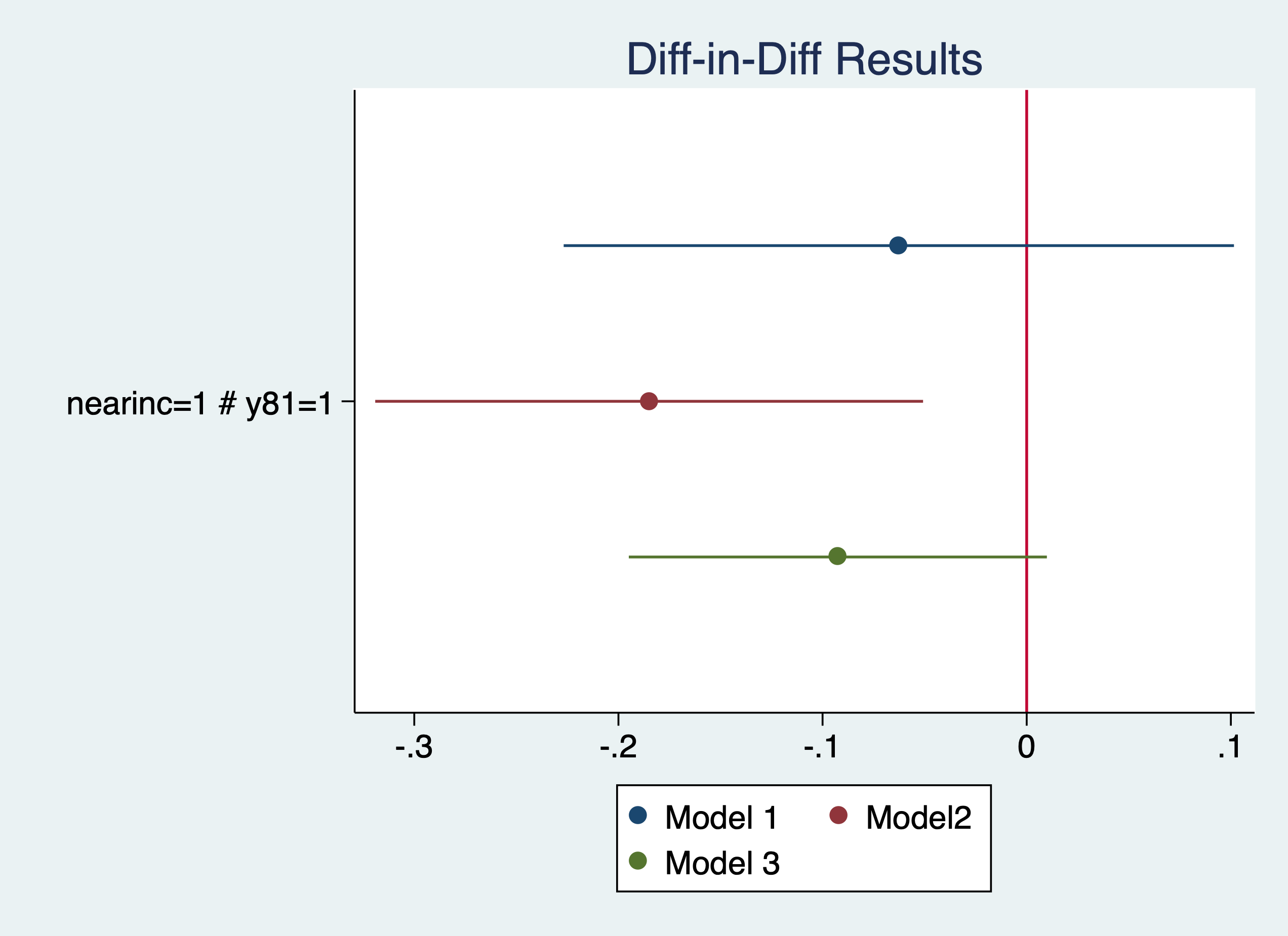
. coefplot (mod1, label(Model 1)) (mod2, label(Model2)) (mod3, label(Model 3)), keep(1.nearinc#1.y81) xline(0) titl
> e("Diff-in-Diff Results")

. graph export "/Users/Sam/Desktop/Econ 645/Stata/week5_housing.png", replace
(file /Users/Sam/Desktop/Econ 645/Stata/week5_housing.png written in PNG format)
More on coefplot https://repec.sowi.unibe.ch/stata/coefplot/getting-started.html
We see that the results are sensitive to the specification. The coefficients range from -6.1% to -16.9%, but their statistical significance varies as well. It would have been helpful to have a larger sample size.
. use "injury.dta", clear
Meyer, Viscusi, and Durbin (1995) studied the length of time that an injured worker receives workers’ compensation (in weeks). On July 15, 1980 Kentucky raised the cap on weekly earnings that were covered by workers’ compensation. An increase in the cap should affect high-wage workers and not affect low-wage workers, so low-wage workers are our control group and high-wage workers are our treatment group.
. tab highearn afchnge

           │        afchnge
  highearn │         0          1 │     Total
───────────┼──────────────────────┼──────────
         0 │     2,294      2,004 │     4,298
         1 │     1,472      1,380 │     2,852
───────────┼──────────────────────┼──────────
     Total │     3,766      3,384 │     7,150
Our diff-in-diff - limited to only KY The policy increased duration of workers’ compensation by 21% to 26%
. reg ldurat i.afchnge##i.highearn if ky==1

      Source │       SS           df       MS      Number of obs   =     5,626
─────────────┼──────────────────────────────────   F(3, 5622)      =     39.54
       Model │  191.071442         3  63.6904807   Prob > F        =    0.0000
    Residual │   9055.9345     5,622  1.61080301   R-squared       =    0.0207
─────────────┼──────────────────────────────────   Adj R-squared   =    0.0201
       Total │  9247.00594     5,625  1.64391217   Root MSE        =    1.2692

─────────────────┬────────────────────────────────────────────────────────────────
          ldurat │      Coef.   Std. Err.      t    P>|t|     [95% Conf. Interval]
─────────────────┼────────────────────────────────────────────────────────────────
       1.afchnge │   .0076573   .0447173     0.17   0.864    -.0800058    .0953204
      1.highearn │   .2564785   .0474464     5.41   0.000     .1634652    .3494918
                 │
afchnge#highearn │
            1 1  │   .1906012   .0685089     2.78   0.005     .0562973    .3249051
                 │
           _cons │   1.125615   .0307368    36.62   0.000     1.065359    1.185871
─────────────────┴────────────────────────────────────────────────────────────────

. reg ldurat i.afchnge##i.highearn i.male i.married i.indust i.injtype if ky==1

      Source │       SS           df       MS      Number of obs   =     5,349
─────────────┼──────────────────────────────────   F(14, 5334)     =     16.37
       Model │  358.441793        14  25.6029852   Prob > F        =    0.0000
    Residual │  8341.41206     5,334  1.56381928   R-squared       =    0.0412
─────────────┼──────────────────────────────────   Adj R-squared   =    0.0387
       Total │  8699.85385     5,348  1.62674904   Root MSE        =    1.2505

─────────────────┬────────────────────────────────────────────────────────────────
          ldurat │      Coef.   Std. Err.      t    P>|t|     [95% Conf. Interval]
─────────────────┼────────────────────────────────────────────────────────────────
       1.afchnge │   .0106274   .0449167     0.24   0.813    -.0774276    .0986824
      1.highearn │   .1757598   .0517462     3.40   0.001     .0743161    .2772035
                 │
afchnge#highearn │
            1 1  │   .2308768   .0695248     3.32   0.001     .0945798    .3671738
                 │
          1.male │  -.0979407   .0445498    -2.20   0.028    -.1852766   -.0106049
       1.married │   .1220995   .0391228     3.12   0.002     .0454027    .1987962
                 │
          indust │
              2  │   .2708676    .058666     4.62   0.000     .1558581     .385877
              3  │   .1606709   .0409038     3.93   0.000     .0804827    .2408591
                 │
         injtype │
              2  │   .7838129    .156167     5.02   0.000     .4776617    1.089964
              3  │   .3353613   .0923382     3.63   0.000     .1543407     .516382
              4  │   .6403517   .1008698     6.35   0.000     .4426058    .8380977
              5  │   .5053036   .0928059     5.44   0.000     .3233661    .6872411
              6  │   .3936092   .0935647     4.21   0.000     .2101841    .5770344
              7  │   .7866121    .207028     3.80   0.000     .3807527    1.192472
              8  │   .5139003   .1292776     3.98   0.000     .2604634    .7673372
                 │
           _cons │   .5713505     .10266     5.57   0.000     .3700949    .7726061
─────────────────┴────────────────────────────────────────────────────────────────
Not in Wooldridge: Is this an appropriate comparison group? I would say no, but high earners vs low earners would be appropriate if we wanted to test a triple difference.
A triple DDD a way to test our DD - Placebo test We would expect high earners in KY to have an increase in duration but not other states. We want to check to make sure low earners are not affected by the policy change
Our DD estimate i.afchgne#i.highearn is about the same but not statistically significant. Furthermore, our high earners in KY after the policy are not affected, so our original DD design might not be rigourous enough.
. reg ldurat i.afchnge##i.highearn##i.ky

      Source │       SS           df       MS      Number of obs   =     7,150
─────────────┼──────────────────────────────────   F(7, 7142)      =     26.09
       Model │  305.206353         7  43.6009075   Prob > F        =    0.0000
    Residual │  11935.9043     7,142  1.67122715   R-squared       =    0.0249
─────────────┼──────────────────────────────────   Adj R-squared   =    0.0240
       Total │  12241.1107     7,149  1.71228293   Root MSE        =    1.2928

────────────────────┬────────────────────────────────────────────────────────────────
             ldurat │      Coef.   Std. Err.      t    P>|t|     [95% Conf. Interval]
────────────────────┼────────────────────────────────────────────────────────────────
          1.afchnge │   .0973808   .0796305     1.22   0.221    -.0587186    .2534802
         1.highearn │   .1691388   .0991463     1.71   0.088    -.0252172    .3634948
                    │
   afchnge#highearn │
               1 1  │   .1919906   .1447922     1.33   0.185    -.0918449    .4758262
                    │
               1.ky │  -.2871215   .0617866    -4.65   0.000    -.4082416   -.1660014
                    │
         afchnge#ky │
               1 1  │  -.0897235   .0917369    -0.98   0.328     -.269555     .090108
                    │
        highearn#ky │
               1 1  │   .0873397   .1102977     0.79   0.428    -.1288765     .303556
                    │
afchnge#highearn#ky │
             1 1 1  │  -.0013894   .1607305    -0.01   0.993    -.3164689      .31369
                    │
              _cons │   1.412737   .0532672    26.52   0.000     1.308317    1.517156
────────────────────┴────────────────────────────────────────────────────────────────

. reg ldurat i.afchnge##i.highearn##i.ky i.male i.married i.indust i.injtype

      Source │       SS           df       MS      Number of obs   =     6,824
─────────────┼──────────────────────────────────   F(18, 6805)     =     18.54
       Model │  541.162741        18  30.0645967   Prob > F        =    0.0000
    Residual │  11032.8204     6,805  1.62128147   R-squared       =    0.0468
─────────────┼──────────────────────────────────   Adj R-squared   =    0.0442
       Total │  11573.9832     6,823   1.6963188   Root MSE        =    1.2733

────────────────────┬────────────────────────────────────────────────────────────────
             ldurat │      Coef.   Std. Err.      t    P>|t|     [95% Conf. Interval]
────────────────────┼────────────────────────────────────────────────────────────────
          1.afchnge │   .0827475    .079902     1.04   0.300    -.0738854    .2393804
         1.highearn │   .1221972   .1003454     1.22   0.223    -.0745112    .3189055
                    │
   afchnge#highearn │
               1 1  │   .1284847   .1448497     0.89   0.375     -.155466    .4124354
                    │
               1.ky │  -.3143542   .0625179    -5.03   0.000    -.4369089   -.1917995
                    │
         afchnge#ky │
               1 1  │  -.0722899   .0921073    -0.78   0.433     -.252849    .1082691
                    │
        highearn#ky │
               1 1  │   .0689824    .110881     0.62   0.534    -.1483789    .2863438
                    │
afchnge#highearn#ky │
             1 1 1  │   .1068157   .1612465     0.66   0.508    -.2092779    .4229093
                    │
             1.male │  -.1501867   .0406318    -3.70   0.000    -.2298379   -.0705356
          1.married │   .1123736   .0349374     3.22   0.001     .0438852    .1808619
                    │
             indust │
                 2  │   .3311585   .0510768     6.48   0.000     .2310319    .4312851
                 3  │   .1485384   .0362317     4.10   0.000     .0775128    .2195639
                    │
            injtype │
                 2  │    .743044    .143936     5.16   0.000     .4608844    1.025204
                 3  │   .3823176   .0852825     4.48   0.000     .2151373     .549498
                 4  │   .6882625   .0923365     7.45   0.000      .507254     .869271
                 5  │    .470878   .0858058     5.49   0.000     .3026718    .6390842
                 6  │   .4012535   .0864441     4.64   0.000     .2317961    .5707109
                 7  │    .923648    .174211     5.30   0.000       .58214    1.265156
                 8  │   .5755271   .1166551     4.93   0.000     .3468466    .8042077
                    │
              _cons │   .9102316   .1051194     8.66   0.000     .7041647    1.116299
────────────────────┴────────────────────────────────────────────────────────────────
Questions: Are worker compensation trends similar between low earners and high earners? Why or why not? Would Michigan make a good comparison group? Can we test this?
. use "kielmc.dta", clear
What is a potential problem with using a binary variable (nearinc) a continuous variable (dist)?
Estimate log(price)=a + b1y81 + b2nearinc + dy81nearinc Do a sensitivity test using additional covariates. Are the results robust, or are they sensitive to the specification? Plot the coefficients of the model.
. use "injury.dta", clear
Estimate log(durat)=a + b1afchnge + b2highearn + dafchngehighearn Do a sensitivity tests using additional covariates. Are the results robust, or Are they sensitive to the specification? Plot the coefficients of the model.
. use "traffic1_reshaped.dta", clear
Set a panel data for the states for 1985 and 1990. You cannot set a panel data set when the unit of analysis is in a string format. Don’t forget the delta option. Use a first differenced equation. Estimate d.thrte=a + b1d.open + b2d.admn Do you get the same results as above? Now try a sensitivity analysis with additional covariates.
. cd "/Users/Sam/Desktop/Econ 645/Data/Mitchell"
/Users/Sam/Desktop/Econ 645/Data/Mitchell
Appending and merging datasets are a crucial part of learning Stata. Many times we are merging datasets by State FIPS, year, Zip Codes, Unit ID, County FIPS, etc. If we wanted to analyze local-level unemployment data to our analysis of county-level crime, then we will likely be using data from BLS and data from FBI or other local admin data.
Note: Working with multiple datasets: I do not have frames in Stata 14, but using frames is encouraged. Using the temp files workaround is a bit cumbersome (but it works). Using Stata frames will help work with those datasets simultaneously to get them ready to merge.
Let’s say we have two datasets with the same variables. We can append these files together using the append command.
. use "moms.dta", clear

. list

     ┌─────────────────────────┐
     │ famid   age   race   hs │
     ├─────────────────────────┤
  1. │     3    24      2    1 │
  2. │     2    28      1    1 │
  3. │     4    21      1    0 │
  4. │     1    33      2    1 │
     └─────────────────────────┘

. use "dads.dta", clear

. list

     ┌─────────────────────────┐
     │ famid   age   race   hs │
     ├─────────────────────────┤
  1. │     1    21      1    0 │
  2. │     4    25      2    1 │
  3. │     2    25      1    1 │
  4. │     3    31      2    1 │
     └─────────────────────────┘
We can append the mom.dta file with append using filename
. append using "moms.dta"

. list

     ┌─────────────────────────┐
     │ famid   age   race   hs │
     ├─────────────────────────┤
  1. │     1    21      1    0 │
  2. │     4    25      2    1 │
  3. │     2    25      1    1 │
  4. │     3    31      2    1 │
  5. │     3    24      2    1 │
     ├─────────────────────────┤
  6. │     2    28      1    1 │
  7. │     4    21      1    0 │
  8. │     1    33      2    1 │
     └─────────────────────────┘
Or,
. clear

. append using "moms.dta" "dads.dta"

. list

     ┌─────────────────────────┐
     │ famid   age   race   hs │
     ├─────────────────────────┤
  1. │     3    24      2    1 │
  2. │     2    28      1    1 │
  3. │     4    21      1    0 │
  4. │     1    33      2    1 │
  5. │     1    21      1    0 │
     ├─────────────────────────┤
  6. │     4    25      2    1 │
  7. │     2    25      1    1 │
  8. │     3    31      2    1 │
     └─────────────────────────┘
What is a clear problem here? After the append, how do we identify which data are for dads and for moms. There are two ways. One, we can generate a variable in both files and code it. Or, we can use the generate option in the append
. clear

. append using "moms.dta" "dads.dta", generate(datascreen)

. list, sepby(datascreen)

     ┌────────────────────────────────────┐
     │ datasc~n   famid   age   race   hs │
     ├────────────────────────────────────┤
  1. │        1       3    24      2    1 │
  2. │        1       2    28      1    1 │
  3. │        1       4    21      1    0 │
  4. │        1       1    33      2    1 │
     ├────────────────────────────────────┤
  5. │        2       1    21      1    0 │
  6. │        2       4    25      2    1 │
  7. │        2       2    25      1    1 │
  8. │        2       3    31      2    1 │
     └────────────────────────────────────┘
Since moms.dta is first, the new variable datascreen will set moms.dta datascreen variable = 1, and since dads.dta is second, the datascreen variable = 2. You could just generate a variable called parent in both files and set moms equal to 1 and dads equal to 0. But, the generate option is nice and concise
It’s a good idea to label the data
. label define datascreenl 1 "From moms.dta" 2 "From dads.dta"

. label values datascreen datascreenl

. list, sepby(datascreen)

     ┌─────────────────────────────────────────┐
     │    datascreen   famid   age   race   hs │
     ├─────────────────────────────────────────┤
  1. │ From moms.dta       3    24      2    1 │
  2. │ From moms.dta       2    28      1    1 │
  3. │ From moms.dta       4    21      1    0 │
  4. │ From moms.dta       1    33      2    1 │
     ├─────────────────────────────────────────┤
  5. │ From dads.dta       1    21      1    0 │
  6. │ From dads.dta       4    25      2    1 │
  7. │ From dads.dta       2    25      1    1 │
  8. │ From dads.dta       3    31      2    1 │
     └─────────────────────────────────────────┘
If we use the generate option in append with one file open, the values of the generated variable are different
. clear

. use "moms.dta"

. append using "dads.dta", generate(datascreen)

. list, sepby(datascreen)

     ┌────────────────────────────────────┐
     │ famid   age   race   hs   datasc~n │
     ├────────────────────────────────────┤
  1. │     3    24      2    1          0 │
  2. │     2    28      1    1          0 │
  3. │     4    21      1    0          0 │
  4. │     1    33      2    1          0 │
     ├────────────────────────────────────┤
  5. │     1    21      1    0          1 │
  6. │     4    25      2    1          1 │
  7. │     2    25      1    1          1 │
  8. │     3    31      2    1          1 │
     └────────────────────────────────────┘

. label define datascreenl 0 "From moms.dta" 1 "From dads.dta"

. label values datascreen datascreenl

. list, sepby(datascreen)

     ┌─────────────────────────────────────────┐
     │ famid   age   race   hs      datascreen │
     ├─────────────────────────────────────────┤
  1. │     3    24      2    1   From moms.dta │
  2. │     2    28      1    1   From moms.dta │
  3. │     4    21      1    0   From moms.dta │
  4. │     1    33      2    1   From moms.dta │
     ├─────────────────────────────────────────┤
  5. │     1    21      1    0   From dads.dta │
  6. │     4    25      2    1   From dads.dta │
  7. │     2    25      1    1   From dads.dta │
  8. │     3    31      2    1   From dads.dta │
     └─────────────────────────────────────────┘
We can append multiple datafiles together (as long as they have the same variables)
. dir br*.dta

-rw-r--r--  1 Sam  staff  2604 Aug 15  2023 br_clarence.dta
-rw-r--r--  1 Sam  staff  2553 Aug 15  2023 br_isaac.dta
-rw-r--r--  1 Sam  staff  2583 Aug 15  2023 br_sally.dta
. use "br_clarence.dta", clear

. list

     ┌──────────────────────────────────────────────────────────────┐
     │ booknum                                        book   rating │
     ├──────────────────────────────────────────────────────────────┤
  1. │       1                   A Fistful of Significance        5 │
  2. │       2    For Whom the Null Hypothesis is Rejected       10 │
  3. │       3   Journey to the Center of the Normal Curve        6 │
     └──────────────────────────────────────────────────────────────┘
. clear

. append using "br_clarence.dta" "br_isaac" "br_sally", generate(rev)

. label define revl 1 "clarence" 2 "isaac" 3 "sally"

. label values rev revl

. list, sepby(rev)

     ┌─────────────────────────────────────────────────────────────────────────┐
     │      rev   booknum                                        book   rating │
     ├─────────────────────────────────────────────────────────────────────────┤
  1. │ clarence         1                   A Fistful of Significance        5 │
  2. │ clarence         2    For Whom the Null Hypothesis is Rejected       10 │
  3. │ clarence         3   Journey to the Center of the Normal Curve        6 │
     ├─────────────────────────────────────────────────────────────────────────┤
  4. │    isaac         1                    The Dreaded Type I Error        6 │
  5. │    isaac         2                           How to Find Power        9 │
  6. │    isaac         3                                The Outliers        8 │
     ├─────────────────────────────────────────────────────────────────────────┤
  7. │    sally         1           Random Effects for Fun and Profit        6 │
  8. │    sally         2                           A Tale of t-tests        9 │
  9. │    sally         3          Days of Correlation and Regression        8 │
     └─────────────────────────────────────────────────────────────────────────┘
We can check the two datasets for potential problems with the precombine command. You will need to install this community-user command. We can check to see if the components of the datasets are similar to prevent problem: variable types, format, labels, values labels, and number of times the variable shows up in the datasets.
. search precombine

. clear

. precombine "moms.dta" "dads.dta", describe(type format varlab vallab ndta) uniquevars

Reports relevant to the combining of the following datasets:
[vars: 4     obs: 4]        moms.dta
[vars: 4     obs: 4]        dads.dta

Variables that appear in multiple datasets:
  ┌─────────────────────────────────────────────────────────────────────────┐
  │ variable    dataset    type   format         varlab   vallabname   ndta │
  ├─────────────────────────────────────────────────────────────────────────┤
  │      age   dads.dta   float    %5.0g            Age                   2 │
  │      age   moms.dta   float    %5.0g            Age                   2 │
  ├─────────────────────────────────────────────────────────────────────────┤
  │    famid   dads.dta   float    %5.0g      Family ID                   2 │
  │    famid   moms.dta   float    %5.0g      Family ID                   2 │
  ├─────────────────────────────────────────────────────────────────────────┤
  │       hs   dads.dta   float    %7.0g   HS Graduate?                   2 │
  │       hs   moms.dta   float    %7.0g   HS Graduate?                   2 │
  ├─────────────────────────────────────────────────────────────────────────┤
  │     race   dads.dta   float    %5.0g           Race                   2 │
  │     race   moms.dta   float    %5.0g      Ethnicity                   2 │
  └─────────────────────────────────────────────────────────────────────────┘

There are no variables that appear in only one dataset,
 i.e. every variable appears in multiple datasets.
If the same variable intent has two different variable names between the data sets, then they will become two different columns when you only want one column of data. For example, when we append moms1 and dads1 which have different variable names for the different variables, the variables do not append correctly.
. use "moms1.dta", clear

. append using "dads1.dta", generate(datascreen)

. list

     ┌────────────────────────────────────────────────────────────┐
     │ famid   mage   mrace   mhs   datasc~n   dage   drace   dhs │
     ├────────────────────────────────────────────────────────────┤
  1. │     1     33       2     1          0      .       .     . │
  2. │     2     28       1     1          0      .       .     . │
  3. │     3     24       2     1          0      .       .     . │
  4. │     4     21       1     0          0      .       .     . │
  5. │     1      .       .     .          1     21       1     0 │
     ├────────────────────────────────────────────────────────────┤
  6. │     2      .       .     .          1     25       1     1 │
  7. │     3      .       .     .          1     31       2     1 │
  8. │     4      .       .     .          1     25       2     1 │
     └────────────────────────────────────────────────────────────┘
It’s an easy fix. Just rename the variables to a common variable name and append
. use "moms1.dta", clear

. rename (mage mrace mhs) (age race hs)

. save "moms1temp.dta", replace
file moms1temp.dta saved
. use "dads1.dta", clear

. rename (dage drace dhs) (age race hs)

. save "dads1temp.dta", replace
file dads1temp.dta saved
. append using "moms1temp.dta" "dads1temp.dta", generate(datascreen)

. list

     ┌────────────────────────────────────┐
     │ famid   age   race   hs   datasc~n │
     ├────────────────────────────────────┤
  1. │     1    21      1    0          0 │
  2. │     2    25      1    1          0 │
  3. │     3    31      2    1          0 │
  4. │     4    25      2    1          0 │
  5. │     1    33      2    1          1 │
     ├────────────────────────────────────┤
  6. │     2    28      1    1          1 │
  7. │     3    24      2    1          1 │
  8. │     4    21      1    0          1 │
  9. │     1    21      1    0          2 │
 10. │     2    25      1    1          2 │
     ├────────────────────────────────────┤
 11. │     3    31      2    1          2 │
 12. │     4    25      2    1          2 │
     └────────────────────────────────────┘
If we have conflicting variable labels, then the variable labels of the primary dataset will overwrite the appended dataset. The solution is to use a neutral variable label. For example, instead of Mom’s HS and Dad’s HS, just have “high school” as the variable label in both datasets
Use neutral variable label names.
. use "momslab.dta", clear

. append using "dadslab.dta", generate(datascreen)
(label eth already defined)

. describe

Contains data from momslab.dta
  obs:             8
 vars:             5                          27 Dec 2009 21:47
 size:           136
───────────────────────────────────────────────────────────────────────────────────────────────────────────────────
              storage   display    value
variable name   type    format     label      variable label
───────────────────────────────────────────────────────────────────────────────────────────────────────────────────
famid           float   %5.0g                 Family ID
age             float   %5.0g                 Mom's Age
race            float   %9.0g      eth        Mom's Ethnicity
hs              float   %15.0g     grad       Is Mom a HS Graduate?
datascreen      byte    %8.0g
───────────────────────────────────────────────────────────────────────────────────────────────────────────────────
Sorted by:
     Note: Dataset has changed since last saved.
. use "momslab.dta", clear

. label variable hs "High School Degree"

. label variable race "Race/Ethnicity"

. label variable age "Age"

. save "momslab1.dta", replace
file momslab1.dta saved
. use "dadslab.dta", clear

. label variable hs "High School Degree"

. label variable race "Race/Ethnicity"

. label variable age "Age"

. save "dadslab1.dta", replace
file dadslab1.dta saved
. use "momslab1.dta", clear

. append using "dadslab1.dta", generate(datascreen)
(label eth already defined)

. describe

Contains data from momslab1.dta
  obs:             8
 vars:             5                          13 Apr 2025 15:55
 size:           136
───────────────────────────────────────────────────────────────────────────────────────────────────────────────────
              storage   display    value
variable name   type    format     label      variable label
───────────────────────────────────────────────────────────────────────────────────────────────────────────────────
famid           float   %5.0g                 Family ID
age             float   %5.0g                 Age
race            float   %9.0g      eth        Race/Ethnicity
hs              float   %15.0g     grad       High School Degree
datascreen      byte    %8.0g
───────────────────────────────────────────────────────────────────────────────────────────────────────────────────
Sorted by:
     Note: Dataset has changed since last saved.
. save momsdadlab1.dta, replace
file momsdadlab1.dta saved
Using our previous files, we find that the value labels may also be incorrect when appending. The primary file (the open one) will supersede the values in the appended file.
Note: this will not throw an error and your data will append, but it might be confusing for yourself in the future or for a replicator. It is good practice to use neutral value labels and value label names.
Let’s look at our files again. If you will notice that the value label names and the value labels will rename as the primary dataset’s value label name and value labels’ values.
. use momslab, clear

. codebook race hs

───────────────────────────────────────────────────────────────────────────────────────────────────────────────────
race                                                                                                Mom's Ethnicity
───────────────────────────────────────────────────────────────────────────────────────────────────────────────────

                  type:  numeric (float)
                 label:  eth

                 range:  [1,2]                        units:  1
         unique values:  2                        missing .:  0/4

            tabulation:  Freq.   Numeric  Label
                             2         1  Mom White
                             2         2  Mom Black

───────────────────────────────────────────────────────────────────────────────────────────────────────────────────
hs                                                                                            Is Mom a HS Graduate?
───────────────────────────────────────────────────────────────────────────────────────────────────────────────────

                  type:  numeric (float)
                 label:  grad

                 range:  [0,1]                        units:  1
         unique values:  2                        missing .:  0/4

            tabulation:  Freq.   Numeric  Label
                             1         0  Mom Not HS Grad
                             3         1  Mom HS Grad
. use dadslab, clear

. codebook race hs

───────────────────────────────────────────────────────────────────────────────────────────────────────────────────
race                                                                                                Dad's Ethnicity
───────────────────────────────────────────────────────────────────────────────────────────────────────────────────

                  type:  numeric (float)
                 label:  eth

                 range:  [1,2]                        units:  1
         unique values:  2                        missing .:  0/4

            tabulation:  Freq.   Numeric  Label
                             2         1  Dad White
                             2         2  Dad Black

───────────────────────────────────────────────────────────────────────────────────────────────────────────────────
hs                                                                                            Is Dad a HS Graduate?
───────────────────────────────────────────────────────────────────────────────────────────────────────────────────

                  type:  numeric (float)
                 label:  hsgrad

                 range:  [0,1]                        units:  1
         unique values:  2                        missing .:  0/4

            tabulation:  Freq.   Numeric  Label
                             1         0  Dad Not HS Grad
                             3         1  Dad HS Grad
. use "momsdadlab1.dta", replace

. codebook race hs

───────────────────────────────────────────────────────────────────────────────────────────────────────────────────
race                                                                                                 Race/Ethnicity
───────────────────────────────────────────────────────────────────────────────────────────────────────────────────

                  type:  numeric (float)
                 label:  eth

                 range:  [1,2]                        units:  1
         unique values:  2                        missing .:  0/8

            tabulation:  Freq.   Numeric  Label
                             4         1  Mom White
                             4         2  Mom Black

───────────────────────────────────────────────────────────────────────────────────────────────────────────────────
hs                                                                                               High School Degree
───────────────────────────────────────────────────────────────────────────────────────────────────────────────────

                  type:  numeric (float)
                 label:  grad

                 range:  [0,1]                        units:  1
         unique values:  2                        missing .:  0/8

            tabulation:  Freq.   Numeric  Label
                             2         0  Mom Not HS Grad
                             6         1  Mom HS Grad
You will notice that the value label name in the dads file is hsgrad, while the moms file is grad. Grad supersedes the value label name hsgrad in the dads file. You will also notice that when you describe the data, a message for the value labels will say eth (which is the same for both), but all the data say Mom White or Mom Black.
Use neutral value labels and neutral value label names.
Another problem that will not throw an error, but it will cause problems are inconsistent variable coding. If we have a binary variable for high school degree or note, where one data set is 0-No and 1-Yes and the other is 1-No 2-Yes, an error will not be thrown when the datasets are appended. However, it will be a problem if you try to use a factor variable, since there conflicting and inconsistent coding.
Check your data, and check the data dictionaries of all the datasets. Summarize and tabulate your data by the datasets after appending will help prevent this. When you find the issue, just recode the variables to be consistent
. use "momshs.dta", clear

. append using "dads.dta", gen(datascreen)

. list

     ┌────────────────────────────────────┐
     │ famid   age   race   hs   datasc~n │
     ├────────────────────────────────────┤
  1. │     3    24      2    2          0 │
  2. │     2    28      1    2          0 │
  3. │     4    21      1    1          0 │
  4. │     1    33      2    1          0 │
  5. │     1    21      1    0          1 │
     ├────────────────────────────────────┤
  6. │     4    25      2    1          1 │
  7. │     2    25      1    1          1 │
  8. │     3    31      2    1          1 │
     └────────────────────────────────────┘

. tab hs datascreen

        HS │      datascreen
 Graduate? │         0          1 │     Total
───────────┼──────────────────────┼──────────
         0 │         0          1 │         1
         1 │         2          3 │         5
         2 │         2          0 │         2
───────────┼──────────────────────┼──────────
     Total │         4          4 │         8
Just recode the data to be consistent after finding the problem
. use "momshs.dta", clear

. recode hs (1=0) (2=1)
(hs: 4 changes made)
Or replace hs=0 if hs == 1 replace hs=1 if hs == 2
. append using "dads.dta", gen(datascreen)

. tab hs datascreen

        HS │      datascreen
 Graduate? │         0          1 │     Total
───────────┼──────────────────────┼──────────
         0 │         2          1 │         3
         1 │         2          3 │         5
───────────┼──────────────────────┼──────────
     Total │         4          4 │         8
When we try to append data of a different time an error will be thrown. We can use the force option to prevent the error, but as we have seen before this can cause numeric string variables with nonnumeric characters to become missing. This will cause data lose and additional measurement error.
. use "moms.dta", clear

. append using "dadstr.dta", generate(datascreen)
variable hs is float in master but str3 in using data
    You could specify append's force option to ignore this numeric/string mismatch.  The using variable would
    then be treated as if it contained numeric missing value.
Resolve the discrepency in variable type before converting. Destring the string variable containing numeric data in string format. Using force may result in data loss if not properly analyzed beforehand.
. use "dadstr.dta", clear

. destring hs, replace
hs: all characters numeric; replaced as byte

. save "dadstrtemp.dta", replace
file dadstrtemp.dta saved
. use "moms.dta", clear

. append using "dadstrtemp.dta", gen(datascreen)

. list, sepby(datascreen)

     ┌────────────────────────────────────┐
     │ famid   age   race   hs   datasc~n │
     ├────────────────────────────────────┤
  1. │     3    24      2    1          0 │
  2. │     2    28      1    1          0 │
  3. │     4    21      1    0          0 │
  4. │     1    33      2    1          0 │
     ├────────────────────────────────────┤
  5. │     1    21      1    0          1 │
  6. │     4    25      2    1          1 │
  7. │     2    25      1    1          1 │
  8. │     3    31      2    1          1 │
     └────────────────────────────────────┘
Let’s go back to 6.13 converting strings to numerics.
. use "dadstr.dta", clear
In small datasets, this is easy to check and fix. HOWEVER, in large datasets, you will need different techniques. I found this on Statalist using regular expressions. As I have said before, regular expressions can be a pain, but they are powerful. This statement below extracts the numerics from the string. https://www.statalist.org/forums/forum/general-stata-discussion/general/967675-removing-non-numeric-characters-from-strings regexm() looks for a numerics with “([0-9]+)” from the string hs regexs() looks for the nth part of the string.
. gen n = real(regexs(1)) if regexm(hs,"([0-9]+)")

. list

     ┌─────────────────────────────┐
     │ famid   age   race   hs   n │
     ├─────────────────────────────┤
  1. │     1    21      1    0   0 │
  2. │     4    25      2    1   1 │
  3. │     2    25      1    1   1 │
  4. │     3    31      2    1   1 │
     └─────────────────────────────┘
An example of how regexm and regexs work from the help file
. clear

. input str15 number

              number
  1. "(123) 456-7890"
  2. "(800) STATAPC"
  3. end
. gen str newnum1 = regexs(1) if regexm(number, "^\(([0-9]+)\) (.*)")

. gen str newnum2 = regexs(2) if regexm(number, "^\(([0-9]+)\) (.*)")

. gen str newnum = regexs(1) + "-" + regexs(2) if regexm(number, "^\(([0-9]+)\) (.*)")

. list number newnum

     ┌───────────────────────────────┐
     │         number         newnum │
     ├───────────────────────────────┤
  1. │ (123) 456-7890   123-456-7890 │
  2. │  (800) STATAPC    800-STATAPC │
     └───────────────────────────────┘
regexm can be a lifesaver if you have numerical data stuck in string format with nonnumeric characters in a large file.
Appending is straightforward and relatively easy to check to make sure everything was appended well. Mergering is a bit tricker, since additional problems can occur, along with different types of merging. Our command for merging is merge.
Before discussing merging. It is KEY to have a identifier variable that is common between two datasets if they will merge. Examples include personal id, firm id, state FIPS, county FIPS, zipcode, etc.
You may need multiple variables besides the identifier to properly merge. Let’s say we want to merge state-level employment from the BLS QCEW with state-level GDP from BEA. We will likely need the county 2-digit FIPS code AND a time identifier, such as quarter or year. If the second identifier is missing we will not be able to properly merge the data.
Note: In Stata, there are two datasets when merging. One is called the master dataset and the other is called the using dataset.
From our moms and dads datasets our KEY variable to merge is family id (famid) the moms1 dataset will be the master and the dads1 will be the using dataset
. use moms1, clear

. list

     ┌────────────────────────────┐
     │ famid   mage   mrace   mhs │
     ├────────────────────────────┤
  1. │     1     33       2     1 │
  2. │     2     28       1     1 │
  3. │     3     24       2     1 │
  4. │     4     21       1     0 │
     └────────────────────────────┘
There are only 1 observation per family, so we can do a 1-to-1 match.
. merge 1:1 famid using dads1

    Result                           # of obs.
    ─────────────────────────────────────────
    not matched                             0
    matched                                 4  (_merge==3)
    ─────────────────────────────────────────

. list

     ┌───────────────────────────────────────────────────────────────┐
     │ famid   mage   mrace   mhs   dage   drace   dhs        _merge │
     ├───────────────────────────────────────────────────────────────┤
  1. │     1     33       2     1     21       1     0   matched (3) │
  2. │     2     28       1     1     25       1     1   matched (3) │
  3. │     3     24       2     1     31       2     1   matched (3) │
  4. │     4     21       1     0     25       2     1   matched (3) │
     └───────────────────────────────────────────────────────────────┘
Our focus should be on _merge. If _merge == 3, then that means all of our matches worked. If _merge == 1 or _merge ==2, then we have some non-merged observations. We may want this, or we might not expect this. Either way, it is a good idea to investigate.
Ironically enough, having two different variable names works well with merge compared to append. We now have two variables for hs, race, and age, but with m or d to distinguish moms and dads. You can easily reshape these data into a long format if necessary.
. use "moms2.dta", clear

. merge 1:1 famid using "dads2.dta"

    Result                           # of obs.
    ─────────────────────────────────────────
    not matched                             3
        from master                         2  (_merge==1)
        from using                          1  (_merge==2)

    matched                                 2  (_merge==3)
    ─────────────────────────────────────────
We can see that when we merge, a variable called _merge is created to identify which observations merged and which did not and why (only master, only using). We can tabulate the _merge variable that is created
. codebook _merge

───────────────────────────────────────────────────────────────────────────────────────────────────────────────────
_merge                                                                                                  (unlabeled)
───────────────────────────────────────────────────────────────────────────────────────────────────────────────────

                  type:  numeric (byte)
                 label:  _merge

                 range:  [1,3]                        units:  1
         unique values:  3                        missing .:  0/5

            tabulation:  Freq.   Numeric  Label
                             2         1  master only (1)
                             1         2  using only (2)
                             2         3  matched (3)

. tab _merge

                 _merge │      Freq.     Percent        Cum.
────────────────────────┼───────────────────────────────────
        master only (1) │          2       40.00       40.00
         using only (2) │          1       20.00       60.00
            matched (3) │          2       40.00      100.00
────────────────────────┼───────────────────────────────────
                  Total │          5      100.00
Not every family was in both datasets
. sort famid

. list famid mage mrace dage drace _merge

     ┌───────────────────────────────────────────────────────┐
     │ famid   mage   mrace   dage   drace            _merge │
     ├───────────────────────────────────────────────────────┤
  1. │     1     33       2     21       1       matched (3) │
  2. │     2      .       .     25       1    using only (2) │
  3. │     3     24       2      .       .   master only (1) │
  4. │     4     21       1     25       2       matched (3) │
  5. │     5     39       2      .       .   master only (1) │
     └───────────────────────────────────────────────────────┘
We have two matches between the data set, only 1 non-match that was only in the using data set (_merge==2), and 2 non-matches that were only in the master dataset (_merge==1).
It is a good idea to investigate why there were no matches between the master and using datasets. We may want that or we may not want depending upon the goal. We can use a qualifier to look at which variables were only in the master, using, and ones that matched
. list famid mage mrace dage drace _merge if _merge==1

     ┌───────────────────────────────────────────────────────┐
     │ famid   mage   mrace   dage   drace            _merge │
     ├───────────────────────────────────────────────────────┤
  3. │     3     24       2      .       .   master only (1) │
  5. │     5     39       2      .       .   master only (1) │
     └───────────────────────────────────────────────────────┘

. list famid mage mrace dage drace _merge if _merge==2

     ┌──────────────────────────────────────────────────────┐
     │ famid   mage   mrace   dage   drace           _merge │
     ├──────────────────────────────────────────────────────┤
  2. │     2      .       .     25       1   using only (2) │
     └──────────────────────────────────────────────────────┘

. list famid mage mrace dage drace _merge if _merge==3

     ┌───────────────────────────────────────────────────┐
     │ famid   mage   mrace   dage   drace        _merge │
     ├───────────────────────────────────────────────────┤
  1. │     1     33       2     21       1   matched (3) │
  4. │     4     21       1     25       2   matched (3) │
     └───────────────────────────────────────────────────┘
Only famid 1 and 4 had observations in both datasets.
Let’s say if we only want matched observations, and we are not concerned with unmatched observations, then we can keep only when _merge == 3 and drop the non-matched observations.
. keep if _merge == 3
(3 observations deleted)

. list

     ┌─────────────────────────────────────────────────────────────────────────────────────┐
     │ famid   mage   mrace   mhs   fr_moms2   dage   drace   dhs   fr_dads2        _merge │
     ├─────────────────────────────────────────────────────────────────────────────────────┤
  1. │     1     33       2     1          1     21       1     0          1   matched (3) │
  2. │     4     21       1     0          1     25       2     1          1   matched (3) │
     └─────────────────────────────────────────────────────────────────────────────────────┘
What is we have duplicate ids with a 1-to-1 matching?
. use "momsdup.dta", clear

. list

     ┌───────────────────────────────────────┐
     │ famid   mage   mrace   mhs   fr_moms2 │
     ├───────────────────────────────────────┤
  1. │     1     33       2     1          1 │
  2. │     3     24       2     1          1 │
  3. │     4     21       1     0          1 │
  4. │     4     39       2     0          1 │
     └───────────────────────────────────────┘
We have two observations for famid==4 If we use merge 1:1 famid using “dads2.dta”, It will throw an error, since famid does not unique identify units for matching. You would want to double check that famid is supposed to have two observations before proceeding.
In our prior example we had duplicate for famid, and we might expect that if we had multiple family members. But, for 1-to-1 matching, we need a unique identifier(s) to properly match. Let’s use kids1 for multiple kids for the same family
. use "kids1.dta", clear

. sort famid kidid

. list

     ┌─────────────────────────────┐
     │ famid   kidid   kage   kfem │
     ├─────────────────────────────┤
  1. │     1       1      3      1 │
  2. │     2       1      8      0 │
  3. │     2       2      3      1 │
  4. │     3       1      4      1 │
  5. │     3       2      7      0 │
     ├─────────────────────────────┤
  6. │     4       1      1      0 │
  7. │     4       2      3      0 │
  8. │     4       3      7      0 │
     └─────────────────────────────┘
We now have a family id (famid) and kid id (kidid)
. use "kidname.dta", clear

. sort famid kidid

. list

     ┌───────────────────────┐
     │ famid   kidid   kname │
     ├───────────────────────┤
  1. │     1       1     Sue │
  2. │     2       1     Vic │
  3. │     2       2     Flo │
  4. │     3       1     Ivy │
  5. │     3       2     Abe │
     ├───────────────────────┤
  6. │     4       1     Tom │
  7. │     4       2     Bob │
  8. │     4       3     Cam │
     └───────────────────────┘
Let’s merge using two key matching variable
. use "kids1.dta", clear

. merge 1:1 famid kidid using "kidname.dta"

    Result                           # of obs.
    ─────────────────────────────────────────
    not matched                             0
    matched                                 8  (_merge==3)
    ─────────────────────────────────────────

. list

     ┌───────────────────────────────────────────────────┐
     │ famid   kidid   kage   kfem   kname        _merge │
     ├───────────────────────────────────────────────────┤
  1. │     1       1      3      1     Sue   matched (3) │
  2. │     2       1      8      0     Vic   matched (3) │
  3. │     2       2      3      1     Flo   matched (3) │
  4. │     3       1      4      1     Ivy   matched (3) │
  5. │     3       2      7      0     Abe   matched (3) │
     ├───────────────────────────────────────────────────┤
  6. │     4       1      1      0     Tom   matched (3) │
  7. │     4       2      3      0     Bob   matched (3) │
  8. │     4       3      7      0     Cam   matched (3) │
     └───────────────────────────────────────────────────┘
Sometimes we need to match file’s observations to multiple observations in another data set. Maybe we have CPS data and we want to merge unemployment rates at the state-level to individuals units within those states. We have one values at the state-level for month m that needs to match multilple individuals in state s.
When we have multiple to one observation, we cannot use 1-to-1 merge. We need a 1:m merge. We can illustrate this with moms1.dta and kids1.dta. One mom may have multiple kids, so when we merge kids and moms data, we will need a 1:m merge
. use "moms1.dta", clear

. list

     ┌────────────────────────────┐
     │ famid   mage   mrace   mhs │
     ├────────────────────────────┤
  1. │     1     33       2     1 │
  2. │     2     28       1     1 │
  3. │     3     24       2     1 │
  4. │     4     21       1     0 │
     └────────────────────────────┘

. use "kids1.dta", clear

. list

     ┌─────────────────────────────┐
     │ famid   kidid   kage   kfem │
     ├─────────────────────────────┤
  1. │     3       1      4      1 │
  2. │     3       2      7      0 │
  3. │     2       1      8      0 │
  4. │     2       2      3      1 │
  5. │     4       1      1      0 │
     ├─────────────────────────────┤
  6. │     4       2      3      0 │
  7. │     4       3      7      0 │
  8. │     1       1      3      1 │
     └─────────────────────────────┘
Each kid and mom has a family id (famid) that we will use to match multiple kids to moms. Our moms have 1 observation while the kids have m observations. Since our moms have 1 observation and there are multiple kids, we need to align our 1:m properly. Since moms is the master the 1 is one the left of 1:m, while the using kids has multiple obervations to family it is the m of 1:m.
. use "moms1.dta", clear

. merge 1:m famid using "kids1.dta"

    Result                           # of obs.
    ─────────────────────────────────────────
    not matched                             0
    matched                                 8  (_merge==3)
    ─────────────────────────────────────────

. list

     ┌────────────────────────────────────────────────────────────────┐
     │ famid   mage   mrace   mhs   kidid   kage   kfem        _merge │
     ├────────────────────────────────────────────────────────────────┤
  1. │     1     33       2     1       1      3      1   matched (3) │
  2. │     2     28       1     1       1      8      0   matched (3) │
  3. │     3     24       2     1       2      7      0   matched (3) │
  4. │     4     21       1     0       2      3      0   matched (3) │
  5. │     2     28       1     1       2      3      1   matched (3) │
     ├────────────────────────────────────────────────────────────────┤
  6. │     3     24       2     1       1      4      1   matched (3) │
  7. │     4     21       1     0       1      1      0   matched (3) │
  8. │     4     21       1     0       3      7      0   matched (3) │
     └────────────────────────────────────────────────────────────────┘
If we were using kids as the master
. use "kids1.dta", clear

. merge m:1 famid using "moms1.dta"

    Result                           # of obs.
    ─────────────────────────────────────────
    not matched                             0
    matched                                 8  (_merge==3)
    ─────────────────────────────────────────

. list, sepby(famid)

     ┌────────────────────────────────────────────────────────────────┐
     │ famid   kidid   kage   kfem   mage   mrace   mhs        _merge │
     ├────────────────────────────────────────────────────────────────┤
  1. │     1       1      3      1     33       2     1   matched (3) │
     ├────────────────────────────────────────────────────────────────┤
  2. │     2       1      8      0     28       1     1   matched (3) │
  3. │     2       2      3      1     28       1     1   matched (3) │
     ├────────────────────────────────────────────────────────────────┤
  4. │     3       2      7      0     24       2     1   matched (3) │
  5. │     3       1      4      1     24       2     1   matched (3) │
     ├────────────────────────────────────────────────────────────────┤
  6. │     4       3      7      0     21       1     0   matched (3) │
  7. │     4       2      3      0     21       1     0   matched (3) │
  8. │     4       1      1      0     21       1     0   matched (3) │
     └────────────────────────────────────────────────────────────────┘
If we tried to use 1 on the kids data and m on the moms side, then an error will be thrown saying that famid does not identify observation in the master dataset.
. use "kids1.dta", clear

. list

     ┌─────────────────────────────┐
     │ famid   kidid   kage   kfem │
     ├─────────────────────────────┤
  1. │     3       1      4      1 │
  2. │     3       2      7      0 │
  3. │     2       1      8      0 │
  4. │     2       2      3      1 │
  5. │     4       1      1      0 │
     ├─────────────────────────────┤
  6. │     4       2      3      0 │
  7. │     4       3      7      0 │
  8. │     1       1      3      1 │
     └─────────────────────────────┘

. use moms1.dta, clear

. list

     ┌────────────────────────────┐
     │ famid   mage   mrace   mhs │
     ├────────────────────────────┤
  1. │     1     33       2     1 │
  2. │     2     28       1     1 │
  3. │     3     24       2     1 │
  4. │     4     21       1     0 │
     └────────────────────────────┘
If we use merge 1:m famid using “moms1.dta”, an error will be thrown
1:m means one-to-many - 1 in master, many in using m:1 means many-to-one - many in master, 1 in using Make sure your data are properly ordered in the merge command.
Many times our data are not so clean for a perfect match, so what happens when not all observations in both files have the same identifier (ex: famid)? Let’s use data without all of the same identifiers.
. use "moms2.dta", clear

. list

     ┌───────────────────────────────────────┐
     │ famid   mage   mrace   mhs   fr_moms2 │
     ├───────────────────────────────────────┤
  1. │     1     33       2     1          1 │
  2. │     3     24       2     1          1 │
  3. │     4     21       1     0          1 │
  4. │     5     39       2     0          1 │
     └───────────────────────────────────────┘
. use "kids2.dta", clear

. list, sepby(famid)

     ┌─────────────────────────────┐
     │ famid   kidid   kage   kfem │
     ├─────────────────────────────┤
  1. │     2       2      3      1 │
  2. │     2       1      8      0 │
     ├─────────────────────────────┤
  3. │     3       2      7      0 │
  4. │     3       1      4      1 │
     ├─────────────────────────────┤
  5. │     4       2      3      0 │
  6. │     4       3      7      0 │
  7. │     4       1      1      0 │
     └─────────────────────────────┘
Merge 1-to-many
. use "moms2.dta", clear

. merge 1:m famid using "kids2.dta"

    Result                           # of obs.
    ─────────────────────────────────────────
    not matched                             4
        from master                         2  (_merge==1)
        from using                          2  (_merge==2)

    matched                                 5  (_merge==3)
    ─────────────────────────────────────────
We have 5 matched observations and 4 unmatched observations. 2 observations were only in the moms dataset and 2 observations were in the kids dataset.
. tab _merge

                 _merge │      Freq.     Percent        Cum.
────────────────────────┼───────────────────────────────────
        master only (1) │          2       22.22       22.22
         using only (2) │          2       22.22       44.44
            matched (3) │          5       55.56      100.00
────────────────────────┼───────────────────────────────────
                  Total │          9      100.00

. sort famid kidid

. list, sepby(famid)

     ┌───────────────────────────────────────────────────────────────────────────────┐
     │ famid   mage   mrace   mhs   fr_moms2   kidid   kage   kfem            _merge │
     ├───────────────────────────────────────────────────────────────────────────────┤
  1. │     1     33       2     1          1       .      .      .   master only (1) │
     ├───────────────────────────────────────────────────────────────────────────────┤
  2. │     2      .       .     .          .       1      8      0    using only (2) │
  3. │     2      .       .     .          .       2      3      1    using only (2) │
     ├───────────────────────────────────────────────────────────────────────────────┤
  4. │     3     24       2     1          1       1      4      1       matched (3) │
  5. │     3     24       2     1          1       2      7      0       matched (3) │
     ├───────────────────────────────────────────────────────────────────────────────┤
  6. │     4     21       1     0          1       1      1      0       matched (3) │
  7. │     4     21       1     0          1       2      3      0       matched (3) │
  8. │     4     21       1     0          1       3      7      0       matched (3) │
     ├───────────────────────────────────────────────────────────────────────────────┤
  9. │     5     39       2     0          1       .      .      .   master only (1) │
     └───────────────────────────────────────────────────────────────────────────────┘
When _merge==1 we have missing observations in the kids variables, and when _merge==2 we have missing observations in the moms variables. Non-matched data
. list if _merge == 1 | _merge == 2, sepby(famid)

     ┌───────────────────────────────────────────────────────────────────────────────┐
     │ famid   mage   mrace   mhs   fr_moms2   kidid   kage   kfem            _merge │
     ├───────────────────────────────────────────────────────────────────────────────┤
  1. │     1     33       2     1          1       .      .      .   master only (1) │
     ├───────────────────────────────────────────────────────────────────────────────┤
  2. │     2      .       .     .          .       1      8      0    using only (2) │
  3. │     2      .       .     .          .       2      3      1    using only (2) │
     ├───────────────────────────────────────────────────────────────────────────────┤
  9. │     5     39       2     0          1       .      .      .   master only (1) │
     └───────────────────────────────────────────────────────────────────────────────┘
Matched data
. list if _merge == 3, sepby(famid)

     ┌───────────────────────────────────────────────────────────────────────────┐
     │ famid   mage   mrace   mhs   fr_moms2   kidid   kage   kfem        _merge │
     ├───────────────────────────────────────────────────────────────────────────┤
  4. │     3     24       2     1          1       1      4      1   matched (3) │
  5. │     3     24       2     1          1       2      7      0   matched (3) │
     ├───────────────────────────────────────────────────────────────────────────┤
  6. │     4     21       1     0          1       1      1      0   matched (3) │
  7. │     4     21       1     0          1       2      3      0   matched (3) │
  8. │     4     21       1     0          1       3      7      0   matched (3) │
     └───────────────────────────────────────────────────────────────────────────┘
Sometimes we need to merge more than 2 datasets together. The examples in the book have nogenerate in the merge command. I don’t recommend this, and after you have inspected your first merge and are satisfied with the results use the drop command to drop _merge, and then proceed with your second merge.
Let’s say we have three datasets
. use "moms2.dta", clear

. merge 1:1 famid using "momsbest2.dta"

    Result                           # of obs.
    ─────────────────────────────────────────
    not matched                             3
        from master                         2  (_merge==1)
        from using                          1  (_merge==2)

    matched                                 2  (_merge==3)
    ─────────────────────────────────────────

. sort famid

. list, sepby(famid)

     ┌────────────────────────────────────────────────────────────────────────────┐
     │ famid   mage   mrace   mhs   fr_moms2   mbage   fr_mo~t2            _merge │
     ├────────────────────────────────────────────────────────────────────────────┤
  1. │     1     33       2     1          1       .          .   master only (1) │
     ├────────────────────────────────────────────────────────────────────────────┤
  2. │     2      .       .     .          .      29          1    using only (2) │
     ├────────────────────────────────────────────────────────────────────────────┤
  3. │     3     24       2     1          1      23          1       matched (3) │
     ├────────────────────────────────────────────────────────────────────────────┤
  4. │     4     21       1     0          1      37          1       matched (3) │
     ├────────────────────────────────────────────────────────────────────────────┤
  5. │     5     39       2     0          1       .          .   master only (1) │
     └────────────────────────────────────────────────────────────────────────────┘
Inspect the merge
. tab _merge

                 _merge │      Freq.     Percent        Cum.
────────────────────────┼───────────────────────────────────
        master only (1) │          2       40.00       40.00
         using only (2) │          1       20.00       60.00
            matched (3) │          2       40.00      100.00
────────────────────────┼───────────────────────────────────
                  Total │          5      100.00
You may want another variable to inspect in the tabulation, which is helpful with large datasets where you cannot eyeball every observation. For example
. tab mage _merge

           │        _merge
       Age │ master on  matched ( │     Total
───────────┼──────────────────────┼──────────
        21 │         0          1 │         1
        24 │         0          1 │         1
        33 │         1          0 │         1
        39 │         1          0 │         1
───────────┼──────────────────────┼──────────
     Total │         2          2 │         4
Drop the _merge after successful inspection
. drop _merge
Merge the 3rd dataset
. merge 1:1 famid using "dads2.dta"

    Result                           # of obs.
    ─────────────────────────────────────────
    not matched                             2
        from master                         2  (_merge==1)
        from using                          0  (_merge==2)

    matched                                 3  (_merge==3)
    ─────────────────────────────────────────
Inspect the merge
. tab _merge

                 _merge │      Freq.     Percent        Cum.
────────────────────────┼───────────────────────────────────
        master only (1) │          2       40.00       40.00
            matched (3) │          3       60.00      100.00
────────────────────────┼───────────────────────────────────
                  Total │          5      100.00
Drop the 2nd merge for 3rd merge
. drop _merge
Merge the 4th dataset
. merge 1:1 famid using "dadsandbest.dta"

    Result                           # of obs.
    ─────────────────────────────────────────
    not matched                             1
        from master                         1  (_merge==1)
        from using                          0  (_merge==2)

    matched                                 4  (_merge==3)
    ─────────────────────────────────────────
Inspect the merge
. sort famid

. list famid fr_*, sepby(famid)

     ┌───────────────────────────────────────────────────┐
     │ famid   fr_moms2   fr_mo~t2   fr_dads2   fr_da~t2 │
     ├───────────────────────────────────────────────────┤
  1. │     1          1          .          1          1 │
     ├───────────────────────────────────────────────────┤
  2. │     2          .          1          1          1 │
     ├───────────────────────────────────────────────────┤
  3. │     3          1          1          .          1 │
     ├───────────────────────────────────────────────────┤
  4. │     4          1          1          1          1 │
     ├───────────────────────────────────────────────────┤
  5. │     5          1          .          .          . │
     └───────────────────────────────────────────────────┘
Drop for 4th merge
. drop _merge
Now add a 4th merge but with a 1-to-many
. merge 1:m famid using "kidname.dta"

    Result                           # of obs.
    ─────────────────────────────────────────
    not matched                             1
        from master                         1  (_merge==1)
        from using                          0  (_merge==2)

    matched                                 8  (_merge==3)
    ─────────────────────────────────────────
Inspect the merge
. tab _merge

                 _merge │      Freq.     Percent        Cum.
────────────────────────┼───────────────────────────────────
        master only (1) │          1       11.11       11.11
            matched (3) │          8       88.89      100.00
────────────────────────┼───────────────────────────────────
                  Total │          9      100.00

. list famid fr_*, sepby(famid)

     ┌───────────────────────────────────────────────────┐
     │ famid   fr_moms2   fr_mo~t2   fr_dads2   fr_da~t2 │
     ├───────────────────────────────────────────────────┤
  1. │     1          1          .          1          1 │
     ├───────────────────────────────────────────────────┤
  2. │     2          .          1          1          1 │
     ├───────────────────────────────────────────────────┤
  3. │     3          1          1          .          1 │
     ├───────────────────────────────────────────────────┤
  4. │     4          1          1          1          1 │
     ├───────────────────────────────────────────────────┤
  5. │     5          1          .          .          . │
     ├───────────────────────────────────────────────────┤
  6. │     2          .          1          1          1 │
     ├───────────────────────────────────────────────────┤
  7. │     3          1          1          .          1 │
     ├───────────────────────────────────────────────────┤
  8. │     4          1          1          1          1 │
  9. │     4          1          1          1          1 │
     └───────────────────────────────────────────────────┘
Mitchell suggests a user-contribution command called dmtablist. You must have Stata 16 or higher, so I’m unable to demonstrate it.
There is an interesting update option with the merge if for some reason, you wanted to check an older version of your data. It will replace the data in your master file with data in your using file. I have never used this set of options, but they may have value in future situations.
. use moms5, clear

. list

     ┌────────────────────────────────┐
     │ famid   mage   mrace   mhsgrad │
     ├────────────────────────────────┤
  1. │     1      .       2         1 │
  2. │     2     82       .         1 │
  3. │     3     24       2         . │
  4. │     4     21       1         0 │
     └────────────────────────────────┘
Here is an updated file with error corrections and previously missing data
. use moms5fixes, clear

. list

     ┌────────────────────────────────┐
     │ famid   mage   mrace   mhsgrad │
     ├────────────────────────────────┤
  1. │     1     33       .         . │
  2. │     2     28       1         . │
  3. │     3      .       .         1 │
     └────────────────────────────────┘
If we use the update option, then it will find matching data, missing data to update, and conflicting data, which are data that match on the key variable, but are of different values
. use moms5, clear

. merge 1:1 famid using moms5fixes, update

    Result                           # of obs.
    ─────────────────────────────────────────
    not matched                             1
        from master                         1  (_merge==1)
        from using                          0  (_merge==2)

    matched                                 3
        not updated                         0  (_merge==3)
        missing updated                     2  (_merge==4)
        nonmissing conflict                 1  (_merge==5)
    ─────────────────────────────────────────
Inspect the merge - We have 1 observation famid==4 that there are no corresponding observations in our using data We have 2 missing data in our master that are updated with data from using We have 1 conflict data between the master and using datasets: 82 vs 28.
. sort famid

. list

     ┌──────────────────────────────────────────────────────────┐
     │ famid   mage   mrace   mhsgrad                    _merge │
     ├──────────────────────────────────────────────────────────┤
  1. │     1     33       2         1       missing updated (4) │
  2. │     2     82       1         1   nonmissing conflict (5) │
  3. │     3     24       2         1       missing updated (4) │
  4. │     4     21       1         0           master only (1) │
     └──────────────────────────────────────────────────────────┘
If we want to update the conflicting data, then we need to the replace option along with the update option
. use moms5, clear

. merge 1:1 famid using moms5fixes, update replace

    Result                           # of obs.
    ─────────────────────────────────────────
    not matched                             1
        from master                         1  (_merge==1)
        from using                          0  (_merge==2)

    matched                                 3
        not updated                         0  (_merge==3)
        missing updated                     2  (_merge==4)
        nonmissing conflict                 1  (_merge==5)
    ─────────────────────────────────────────
Inspect the merge - rember if it is a large data set then tabulation by variables may be more appropriate than list
. sort famid

. list

     ┌──────────────────────────────────────────────────────────┐
     │ famid   mage   mrace   mhsgrad                    _merge │
     ├──────────────────────────────────────────────────────────┤
  1. │     1     33       2         1       missing updated (4) │
  2. │     2     28       1         1   nonmissing conflict (5) │
  3. │     3     24       2         1       missing updated (4) │
  4. │     4     21       1         0           master only (1) │
     └──────────────────────────────────────────────────────────┘
There are some additional options in merge, which may be of interest that we will cover.
The keepusing() option can be helpful when merging two datasets with hundreds of variables. Our data sets here are small, but the CPS, ACS, etc. can have hundreds of variables and we may only want a few additional variables from a using dataset
Let’s say we only want dads age and dads race from our using dataset
. use dads1, clear

. list

     ┌────────────────────────────┐
     │ famid   dage   drace   dhs │
     ├────────────────────────────┤
  1. │     1     21       1     0 │
  2. │     2     25       1     1 │
  3. │     3     31       2     1 │
  4. │     4     25       2     1 │
     └────────────────────────────┘
We can use the keepusing() option to keep dage drace
. use moms1, clear

. merge 1:1 famid using dads1, keepusing(dage drace)

    Result                           # of obs.
    ─────────────────────────────────────────
    not matched                             0
    matched                                 4  (_merge==3)
    ─────────────────────────────────────────

. list

     ┌─────────────────────────────────────────────────────────┐
     │ famid   mage   mrace   mhs   dage   drace        _merge │
     ├─────────────────────────────────────────────────────────┤
  1. │     1     33       2     1     21       1   matched (3) │
  2. │     2     28       1     1     25       1   matched (3) │
  3. │     3     24       2     1     31       2   matched (3) │
  4. │     4     21       1     0     25       2   matched (3) │
     └─────────────────────────────────────────────────────────┘
We do not keep dhs after the merge since we specify dage and drace with the keepusing() option
Another interesting option is assert(), which could be useful in certain situations. If we specify assert(match), Stata will throw an error if all observations are not matched. This may or may not be helpful when inspecting the data post-merge. An option of assert(match master) makes sure that all merges are matched or from the original dataset. More information is on page 247-248.
**
I do not recommend using noreport or nogenerate options, since these are essential for inspecting your merges.
generatekeep() option either. You should inspect your data and then when you are satisfied, you can use the drop command with a qualifier using _merge: drop if _merge == 1 | _merge == 2
Merging can be trickier than appending. Appending is fairly straightfoward, but some of the topics are similar
This is a similar problem to append, but we need different variable names instead of the same variable names. If we have common or the same variable names with merge, then we will lose data. It is important to note that
In our example we have similar columns of data, but with different names except for mom’s age and dad’s age which are both named “age”. For example the race column in moms data is called race, while the race column in dads data is called eth. But, both datasets have age named as age.
. use moms3, clear

. list

     ┌─────────────────────────┐
     │ famid   age   race   hs │
     ├─────────────────────────┤
  1. │     1    33      2    1 │
  2. │     2    28      1    1 │
  3. │     3    24      2    1 │
  4. │     4    21      1    0 │
     └─────────────────────────┘

. use dads3, clear

. list

     ┌────────────────────────────┐
     │ famid   age   eth   gradhs │
     ├────────────────────────────┤
  1. │     1    21     1        0 │
  2. │     2    25     1        1 │
  3. │     3    31     2        1 │
  4. │     4    25     2        1 │
     └────────────────────────────┘

. use moms3, clear

. merge 1:1 famid using dads3

    Result                           # of obs.
    ─────────────────────────────────────────
    not matched                             0
    matched                                 4  (_merge==3)
    ─────────────────────────────────────────
Our merge is successful, but we lost dads age. Note, that are merge appears successful and we will not notice the lost data. This easy to notice in a small dataset, but what about datasets with hundreds of variables? We should inspect our data systematically beforehand to prevent this problem.
There is a helpful command called cf (compare files) that can detect variables that are common/same and different between datasets. Once detected, rename the variable to a name that would make sense e.g: momsage.
. use moms3, clear

. capture cf _all using dads3, all verbose
From the cf command, we want to compare variables and we find that race and hs are not in the master file, but age is and there are 4 mismatched observations. We can easily enough rename our age variable in the master before performing our merge. Our all option will compare all the variables, but if we don’t use this option, only mismatched will appear. There is a verbose option that will give a detailed listing of each observation that differs. verbose is probably not practical when merging data between large datasets.
Notice: our key variable famid does not appear as a mismatch.
Remember, In append, when we had different variable names, we would create new and inconsistent columns of data. In merge we want new variable names to preserve all of our data.
Mitchell recommends that you check out a blog on Merges Gone Bad: https://blog.stata.com/2011/04/18/merging-data-part-1-merges-gone-bad/
. search merges gone bad
This is a similiar but slightly different problem that we saw in append. When there are two value labels of the same name, the master value label name will overwrite the using value label name. A message will pop up, but an error will not be thrown.
In our example, high school has label dhs and label mhs so they are unique, but race is common between moms4 and dads4, and when merging the master label values will overwrite the using.
. use moms4, clear

. merge 1:1 famid using dads4
(label race already defined)

    Result                           # of obs.
    ─────────────────────────────────────────
    not matched                             0
    matched                                 4  (_merge==3)
    ─────────────────────────────────────────

. list famid mrace drace mhs dhs

     ┌───────────────────────────────────────────────────────────────────┐
     │ famid       mrace       drace               mhs               dhs │
     ├───────────────────────────────────────────────────────────────────┤
  1. │     1   Mom Black   Mom White       Mom HS Grad   Dad Not HS Grad │
  2. │     2   Mom White   Mom White       Mom HS Grad       Dad HS Grad │
  3. │     3   Mom Black   Mom Black       Mom HS Grad       Dad HS Grad │
  4. │     4   Mom White   Mom Black   Mom Not HS Grad       Dad HS Grad │
     └───────────────────────────────────────────────────────────────────┘
A message saying “label race already defined”)
. label define dracel 1 "White" 2 "Black"

. label values drace drace1

. list famid mrace drace mhs dhs

     ┌───────────────────────────────────────────────────────────────┐
     │ famid       mrace   drace               mhs               dhs │
     ├───────────────────────────────────────────────────────────────┤
  1. │     1   Mom Black       1       Mom HS Grad   Dad Not HS Grad │
  2. │     2   Mom White       1       Mom HS Grad       Dad HS Grad │
  3. │     3   Mom Black       2       Mom HS Grad       Dad HS Grad │
  4. │     4   Mom White       2   Mom Not HS Grad       Dad HS Grad │
     └───────────────────────────────────────────────────────────────┘
Note: your key variables need to be in the same type numerics or strings. Please check your key variables before merging.
You need to be careful when doing m:m matching, and I don’t think Mitchell even talks about this. It is preferable to have your main dataset as your unique observations (your 1), and your using having multiple observation (your m). There could be situations where you might need it, but it shouldn’t be your default go to for merge
. use moms1, clear

. append using dads1

. sort famid

. list

     ┌─────────────────────────────────────────────────┐
     │ famid   mage   mrace   mhs   dage   drace   dhs │
     ├─────────────────────────────────────────────────┤
  1. │     1      .       .     .     21       1     0 │
  2. │     1     33       2     1      .       .     . │
  3. │     2     28       1     1      .       .     . │
  4. │     2      .       .     .     25       1     1 │
  5. │     3      .       .     .     31       2     1 │
     ├─────────────────────────────────────────────────┤
  6. │     3     24       2     1      .       .     . │
  7. │     4      .       .     .     25       2     1 │
  8. │     4     21       1     0      .       .     . │
     └─────────────────────────────────────────────────┘
An example of a problem with m:m merging. We now have multiple famid ids: one for moms, one for dads. And now if we want to merge kids data, we try a m:m matching since we have multiple parents and multiple kids
. merge m:m famid using kids1

    Result                           # of obs.
    ─────────────────────────────────────────
    not matched                             0
    matched                                 9  (_merge==3)
    ─────────────────────────────────────────

. list

     ┌─────────────────────────────────────────────────────────────────────────────────────┐
     │ famid   mage   mrace   mhs   dage   drace   dhs   kidid   kage   kfem        _merge │
     ├─────────────────────────────────────────────────────────────────────────────────────┤
  1. │     1      .       .     .     21       1     0       1      3      1   matched (3) │
  2. │     1     33       2     1      .       .     .       1      3      1   matched (3) │
  3. │     2     28       1     1      .       .     .       1      8      0   matched (3) │
  4. │     2      .       .     .     25       1     1       2      3      1   matched (3) │
  5. │     3      .       .     .     31       2     1       2      7      0   matched (3) │
     ├─────────────────────────────────────────────────────────────────────────────────────┤
  6. │     3     24       2     1      .       .     .       1      4      1   matched (3) │
  7. │     4      .       .     .     25       2     1       3      7      0   matched (3) │
  8. │     4     21       1     0      .       .     .       1      1      0   matched (3) │
  9. │     4     21       1     0      .       .     .       2      3      0   matched (3) │
     └─────────────────────────────────────────────────────────────────────────────────────┘
We need to be careful, and observe our data for problems. We have a duplicative kidid since famid==1 only has one kid We have a duplicative mom in famid==4 This is likely very problematic.
A better approach would be to merge moms and dads data, and then merge the kids data with a 1:m. A joinby might be preferable here, which will be discussed next
joinby command is similar to the merge command but there are some differences.
There are different types of joinby that can be changed by the unmatched() option. There is inner joinby where unmatched() is left off. This is only the matched observations. There is a left joinby where unmatched(master) is added as an option, and we keep all master observation matched or unmatched and drop all unmatched using observations. There is a right joinby where unmatched(using) is added as an option, and we keep all using observations matched or unmatched and drop all unmatched master observation.
joinby command only keeps matched observations by default, but this can be very problematic. I suggest using the unmatched(master) option as it is a left join. You should probably keep your observations in at least one dataset.
I personally recommend that you use merge instead of joinby, since you have more inspection diagnostics to make sure your data merged properly. But there my be situtations where a left-join is a better option instead of a m:m merge. This usually deals with multiple observations for an id variable such as moms and dads and multiple kids.
We have multiple kids for each family ranging from 1 to 3.
. use kidname, clear

. sort famid kname

. list, sepby(famid)

     ┌───────────────────────┐
     │ famid   kidid   kname │
     ├───────────────────────┤
  1. │     1       1     Sue │
     ├───────────────────────┤
  2. │     2       2     Flo │
  3. │     2       1     Vic │
     ├───────────────────────┤
  4. │     3       2     Abe │
  5. │     3       1     Ivy │
     ├───────────────────────┤
  6. │     4       2     Bob │
  7. │     4       3     Cam │
  8. │     4       1     Tom │
     └───────────────────────┘
We have two parents in each family
. use parname, clear

. sort famid

. list

     ┌──────────────────────────────────┐
     │ famid   mom   age   race   pname │
     ├──────────────────────────────────┤
  1. │     1     0    21      1     Sam │
  2. │     1     1    33      2     Lil │
  3. │     2     1    28      1     Ula │
  4. │     2     0    25      1     Nik │
  5. │     3     1    24      2     Ann │
     ├──────────────────────────────────┤
  6. │     3     0    31      2      Al │
  7. │     4     0    25      2     Ted │
  8. │     4     1    21      1     Bev │
     └──────────────────────────────────┘
We’ll look at an inner join first
. joinby famid using kidname

. sort famid kname pname

. list, sepby(famid kidid)

     ┌──────────────────────────────────────────────────┐
     │ famid   mom   age   race   pname   kidid   kname │
     ├──────────────────────────────────────────────────┤
  1. │     1     1    33      2     Lil       1     Sue │
  2. │     1     0    21      1     Sam       1     Sue │
     ├──────────────────────────────────────────────────┤
  3. │     2     0    25      1     Nik       2     Flo │
  4. │     2     1    28      1     Ula       2     Flo │
     ├──────────────────────────────────────────────────┤
  5. │     2     0    25      1     Nik       1     Vic │
  6. │     2     1    28      1     Ula       1     Vic │
     ├──────────────────────────────────────────────────┤
  7. │     3     0    31      2      Al       2     Abe │
  8. │     3     1    24      2     Ann       2     Abe │
     ├──────────────────────────────────────────────────┤
  9. │     3     0    31      2      Al       1     Ivy │
 10. │     3     1    24      2     Ann       1     Ivy │
     ├──────────────────────────────────────────────────┤
 11. │     4     1    21      1     Bev       2     Bob │
 12. │     4     0    25      2     Ted       2     Bob │
     ├──────────────────────────────────────────────────┤
 13. │     4     1    21      1     Bev       3     Cam │
 14. │     4     0    25      2     Ted       3     Cam │
     ├──────────────────────────────────────────────────┤
 15. │     4     1    21      1     Bev       1     Tom │
 16. │     4     0    25      2     Ted       1     Tom │
     └──────────────────────────────────────────────────┘
Notice we have a family id, but also a parent id in the mom variable (0,1) We can have a left-join, but it will be the same as an inner join. This might be preferable, since not all parents may have kids and we would want to keep their data. We’ll look at a left-join
. use parname, clear

. joinby famid using kidname, unmatched(master)

. sort famid kname pname

. list, sepby(famid kidid)

     ┌──────────────────────────────────────────────────────────────────────────────────┐
     │ famid   mom   age   race   pname                          _merge   kidid   kname │
     ├──────────────────────────────────────────────────────────────────────────────────┤
  1. │     1     1    33      2     Lil   both in master and using data       1     Sue │
  2. │     1     0    21      1     Sam   both in master and using data       1     Sue │
     ├──────────────────────────────────────────────────────────────────────────────────┤
  3. │     2     0    25      1     Nik   both in master and using data       2     Flo │
  4. │     2     1    28      1     Ula   both in master and using data       2     Flo │
     ├──────────────────────────────────────────────────────────────────────────────────┤
  5. │     2     0    25      1     Nik   both in master and using data       1     Vic │
  6. │     2     1    28      1     Ula   both in master and using data       1     Vic │
     ├──────────────────────────────────────────────────────────────────────────────────┤
  7. │     3     0    31      2      Al   both in master and using data       2     Abe │
  8. │     3     1    24      2     Ann   both in master and using data       2     Abe │
     ├──────────────────────────────────────────────────────────────────────────────────┤
  9. │     3     0    31      2      Al   both in master and using data       1     Ivy │
 10. │     3     1    24      2     Ann   both in master and using data       1     Ivy │
     ├──────────────────────────────────────────────────────────────────────────────────┤
 11. │     4     1    21      1     Bev   both in master and using data       2     Bob │
 12. │     4     0    25      2     Ted   both in master and using data       2     Bob │
     ├──────────────────────────────────────────────────────────────────────────────────┤
 13. │     4     1    21      1     Bev   both in master and using data       3     Cam │
 14. │     4     0    25      2     Ted   both in master and using data       3     Cam │
     ├──────────────────────────────────────────────────────────────────────────────────┤
 15. │     4     1    21      1     Bev   both in master and using data       1     Tom │
 16. │     4     0    25      2     Ted   both in master and using data       1     Tom │
     └──────────────────────────────────────────────────────────────────────────────────┘
If you are interested in cross data, it can be found on pages 255-257. The cross command matches each observation in the master dataset to the using dataset.
In our moms and dads data set, we have 4 moms and 4 dads. The cross command will match every possible combination, so we have a 4x4 outcome. This might be of interest, and have some usefulness with combination and permutations, but I have never personally used this.
. use moms1, clear

. cross using dads1

. sort famid

. list, sepby(famid)

     ┌─────────────────────────────────────────────────┐
     │ famid   mage   mrace   mhs   dage   drace   dhs │
     ├─────────────────────────────────────────────────┤
  1. │     1     33       2     1     25       1     1 │
  2. │     1     33       2     1     21       1     0 │
  3. │     1     33       2     1     31       2     1 │
  4. │     1     33       2     1     25       2     1 │
     ├─────────────────────────────────────────────────┤
  5. │     2     28       1     1     25       1     1 │
  6. │     2     28       1     1     31       2     1 │
  7. │     2     28       1     1     25       2     1 │
  8. │     2     28       1     1     21       1     0 │
     ├─────────────────────────────────────────────────┤
  9. │     3     24       2     1     25       1     1 │
 10. │     3     24       2     1     25       2     1 │
 11. │     3     24       2     1     21       1     0 │
 12. │     3     24       2     1     31       2     1 │
     ├─────────────────────────────────────────────────┤
 13. │     4     21       1     0     31       2     1 │
 14. │     4     21       1     0     25       1     1 │
 15. │     4     21       1     0     21       1     0 │
 16. │     4     21       1     0     25       2     1 │
     └─────────────────────────────────────────────────┘