Samuel Rowe Adapted from Wooldridge
. clear

. set more off
*Set Working Directory
. cd "/Users/Sam/Desktop/Econ 645/Data/Wooldridge"
/Users/Sam/Desktop/Econ 645/Data/Wooldridge
. use "wagepan.dta", clear
Set the Panel
. xtset nr year
       panel variable:  nr (strongly balanced)
        time variable:  year, 1980 to 1987
                delta:  1 unit
. eststo OLS: reg lwage c.edu exper expersq i.black i.south i.married i.union i.d8*

      Source │       SS           df       MS      Number of obs   =     4,360
─────────────┼──────────────────────────────────   F(14, 4345)     =     73.43
       Model │  236.577196        14  16.8983712   Prob > F        =    0.0000
    Residual │  999.952446     4,345  .230138653   R-squared       =    0.1913
─────────────┼──────────────────────────────────   Adj R-squared   =    0.1887
       Total │  1236.52964     4,359  .283672779   Root MSE        =    .47973

─────────────┬────────────────────────────────────────────────────────────────
       lwage │      Coef.   Std. Err.      t    P>|t|     [95% Conf. Interval]
─────────────┼────────────────────────────────────────────────────────────────
        educ │   .0895815   .0051762    17.31   0.000     .0794334    .0997295
       exper │   .0665418   .0136722     4.87   0.000     .0397372    .0933463
     expersq │  -.0023832   .0008183    -2.91   0.004    -.0039875   -.0007789
     1.black │  -.1275978   .0236068    -5.41   0.000    -.1738791   -.0813165
     1.south │  -.0529354   .0155534    -3.40   0.001    -.0834281   -.0224428
   1.married │   .1122106   .0157149     7.14   0.000     .0814014    .1430198
     1.union │   .1802554   .0171339    10.52   0.000     .1466642    .2138466
       1.d81 │    .058693   .0303147     1.94   0.053    -.0007393    .1181253
       1.d82 │   .0638086   .0331714     1.92   0.054    -.0012242    .1288414
       1.d83 │   .0633355   .0366129     1.73   0.084    -.0084444    .1351153
       1.d84 │   .0915252   .0400387     2.29   0.022     .0130289    .1700216
       1.d85 │   .1105424   .0432973     2.55   0.011     .0256575    .1954272
       1.d86 │   .1437822   .0463663     3.10   0.002     .0528806    .2346837
       1.d87 │   .1756699   .0493736     3.56   0.000     .0788725    .2724673
       _cons │   .1333638   .0774193     1.72   0.085    -.0184175     .285145
─────────────┴────────────────────────────────────────────────────────────────
If we use FE or FD, we cannot assess race, education, or experience
since they remain constant.
. eststo Within: xtreg lwage c.edu exper expersq i.black i.south i.married i.union i.d8*, fe
note: educ omitted because of collinearity
note: 1.black omitted because of collinearity
note: 1.d87 omitted because of collinearity

Fixed-effects (within) regression               Number of obs     =      4,360
Group variable: nr                              Number of groups  =        545

R-sq:                                           Obs per group:
     within  = 0.1815                                         min =          8
     between = 0.0009                                         avg =        8.0
     overall = 0.0497                                         max =          8

                                                F(11,3804)        =      76.71
corr(u_i, Xb)  = -0.1739                        Prob > F          =     0.0000

─────────────┬────────────────────────────────────────────────────────────────
       lwage │      Coef.   Std. Err.      t    P>|t|     [95% Conf. Interval]
─────────────┼────────────────────────────────────────────────────────────────
        educ │          0  (omitted)
       exper │   .1313318   .0098277    13.36   0.000     .1120638    .1505999
     expersq │  -.0051475   .0007043    -7.31   0.000    -.0065284   -.0037666
     1.black │          0  (omitted)
     1.south │   .1018493   .0479605     2.12   0.034     .0078186      .19588
   1.married │   .0462057   .0183034     2.52   0.012     .0103203     .082091
     1.union │   .0809394   .0193065     4.19   0.000     .0430874    .1187914
       1.d81 │   .0190821   .0203532     0.94   0.349    -.0208222    .0589864
       1.d82 │  -.0117214   .0202191    -0.58   0.562    -.0513627    .0279199
       1.d83 │  -.0425071   .0203126    -2.09   0.036    -.0823318   -.0026825
       1.d84 │  -.0378955   .0203069    -1.87   0.062    -.0777089    .0019179
       1.d85 │  -.0427598   .0202377    -2.11   0.035    -.0824377   -.0030819
       1.d86 │  -.0276303   .0203773    -1.36   0.175    -.0675818    .0123211
       1.d87 │          0  (omitted)
       _cons │   .9952994    .033587    29.63   0.000      .929449     1.06115
─────────────┼────────────────────────────────────────────────────────────────
     sigma_u │  .40924292
     sigma_e │  .35082825
         rho │  .57640294   (fraction of variance due to u_i)
─────────────┴────────────────────────────────────────────────────────────────
F test that all u_i=0: F(544, 3804) = 9.54                   Prob > F = 0.0000
. esttab OLS Within, mtitles se scalars(F r2) drop(0.d* 0.union 0.married)

────────────────────────────────────────────
                      (1)             (2)
                      OLS          Within
────────────────────────────────────────────
educ               0.0896***            0
                (0.00518)             (.)

exper              0.0665***        0.131***
                 (0.0137)       (0.00983)

expersq          -0.00238**      -0.00515***
               (0.000818)      (0.000704)

0.black                 0               0
                      (.)             (.)

1.black            -0.128***            0
                 (0.0236)             (.)

0.south                 0               0
                      (.)             (.)

1.south           -0.0529***        0.102*
                 (0.0156)        (0.0480)

1.married           0.112***       0.0462*
                 (0.0157)        (0.0183)

1.union             0.180***       0.0809***
                 (0.0171)        (0.0193)

1.d81              0.0587          0.0191
                 (0.0303)        (0.0204)

1.d82              0.0638         -0.0117
                 (0.0332)        (0.0202)

1.d83              0.0633         -0.0425*
                 (0.0366)        (0.0203)

1.d84              0.0915*        -0.0379
                 (0.0400)        (0.0203)

1.d85               0.111*        -0.0428*
                 (0.0433)        (0.0202)

1.d86               0.144**       -0.0276
                 (0.0464)        (0.0204)

1.d87               0.176***            0
                 (0.0494)             (.)

_cons               0.133           0.995***
                 (0.0774)        (0.0336)
────────────────────────────────────────────
N                    4360            4360
F                   73.43           76.71
r2                  0.191           0.182
────────────────────────────────────────────
Standard errors in parentheses
* p<0.05, ** p<0.01, *** p<0.001
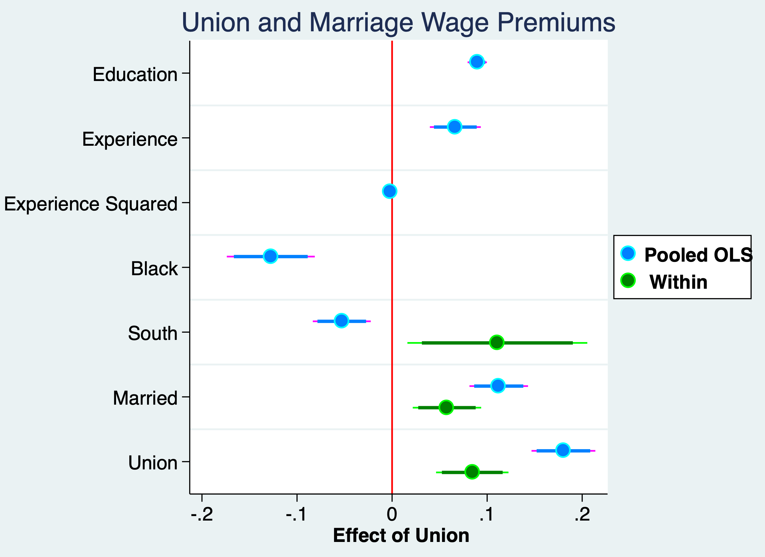
After controlling for time-invariant individual fixed effects the Pooled OLS is seen to be upward biased.
Pooled OLS Wage Premium Estimate
. display (exp(.180)-1)*100
19.721736
FE Within Wage Premium Estimate
. display (exp(.0844)-1)*100
8.8064032
Credit: John Kane: Making Regression Coefficients Plots in Stata
. quietly reg lwage c.edu exper expersq i.black i.south i.married i.union i.d8*

. estimates store pooled

. quietly xtreg lwage c.edu i.black i.south i.married i.union i.d8*, fe

. estimates store fe

. coefplot (pooled, label("{bf:Pooled OLS}") mcolor(midblue) mlcolor(cyan) ///
>   ciopts(lcolor(magenta midblue))) /// options for first group
>   (fe, label("{bf: Within}") mcolor(green) mlcolor(lime) ///
>   ciopts(lcolor(lime green))), /// options for second group
>   title(Union and Marriage Wage Premiums) ///
>   drop(_cons 1.d* 0.black 0.south) ///
>   xline(0, lcolor(red) lwidth(medium)) scheme(jet_white) ///
>   xtitle("{bf: Effect of Union}") ///
>   graphregion(margin(small)) ///
>   coeflabels(educ="Education" exper="Experience" expersq="Experience Squared" ///
>   1.black="Black" 1.south="South" 1.married="Married" ///
>   1.union="Union") ///
>   msize(large) mcolor(%85) mlwidth(medium) msymbol(circle) /// marker options
>   levels(95 90) ciopts(lwidth(medthick thick) recast(rspike rcap)) ///ci options for all groups
>   legend(ring(1) col(1) pos(3) size(medsmall))
(note: scheme jet_white not found, using s2color)

.   graph export "/Users/Sam/Desktop/Econ 645/Stata/week4_union_wage_premium.png", replace
(file /Users/Sam/Desktop/Econ 645/Stata/week4_union_wage_premium.png written in PNG format)
With fixed effects or first differencing, we cannot assess time-invariant variables. Variables that do not vary over time, such as sex, race, or education (assuming) education is static. But, if we interact education with time binaries, we can assess whether returns to education have increased over time.
We can test to see if returns to education are constant over time. use "wagepan.dta", clear
Vella and Verbeek (1998) estimate to see if the returns to education have change over time. We have some variables that are not time-invariant, such as union status and marital status. Experience does growth but it grows at a constant rate. We have a few variable that do not (or we would expect not to change), such as race and education (for older workers)
We use the natural log of wages, which have nice properties, such as being are more normally distributed and providing elasticities. It also can take care of inflation when we add time period binaries.
Set up the Panel
. xtset nr year
       panel variable:  nr (strongly balanced)
        time variable:  year, 1980 to 1987
                delta:  1 unit
. eststo OLS: reg lwage c.edu##i.d8* exper expersq i.married i.union

      Source │       SS           df       MS      Number of obs   =     4,360
─────────────┼──────────────────────────────────   F(19, 4340)     =     50.92
       Model │  225.412805        19  11.8638318   Prob > F        =    0.0000
    Residual │  1011.11684     4,340   .23297623   R-squared       =    0.1823
─────────────┼──────────────────────────────────   Adj R-squared   =    0.1787
       Total │  1236.52964     4,359  .283672779   Root MSE        =    .48268

─────────────┬────────────────────────────────────────────────────────────────
       lwage │      Coef.   Std. Err.      t    P>|t|     [95% Conf. Interval]
─────────────┼────────────────────────────────────────────────────────────────
        educ │    .081673   .0125675     6.50   0.000     .0570343    .1063117
       1.d81 │  -.0356958    .199359    -0.18   0.858    -.4265413    .3551497
       1.d82 │  -.0315288   .1998095    -0.16   0.875    -.4232575       .3602
       1.d83 │  -.0342801   .2007839    -0.17   0.864    -.4279192    .3593589
       1.d84 │   .0242933   .2025167     0.12   0.905    -.3727429    .4213294
       1.d85 │   .0058838   .2052301     0.03   0.977    -.3964719    .4082395
       1.d86 │   .0251586   .2092184     0.12   0.904    -.3850164    .4353336
       1.d87 │   .0372565   .2148364     0.17   0.862    -.3839326    .4584456
             │
  d81#c.educ │
          1  │   .0084448   .0167792     0.50   0.615     -.024451    .0413407
             │
  d82#c.educ │
          1  │   .0088899   .0168742     0.53   0.598    -.0241921     .041972
             │
  d83#c.educ │
          1  │   .0093544   .0170326     0.55   0.583    -.0240381     .042747
             │
  d84#c.educ │
          1  │   .0070671   .0172551     0.41   0.682    -.0267617    .0408958
             │
  d85#c.educ │
          1  │   .0104027   .0175306     0.59   0.553    -.0239662    .0447716
             │
  d86#c.educ │
          1  │   .0116562   .0178614     0.65   0.514    -.0233613    .0466737
             │
  d87#c.educ │
          1  │   .0134166   .0182525     0.74   0.462    -.0223676    .0492008
             │
       exper │   .0568876   .0154436     3.68   0.000     .0266102     .087165
     expersq │   -.001919   .0009455    -2.03   0.042    -.0037726   -.0000654
   1.married │   .1229473   .0155752     7.89   0.000     .0924119    .1534827
     1.union │   .1720565   .0171378    10.04   0.000     .1384575    .2056554
       _cons │   .2175863   .1641736     1.33   0.185    -.1042777    .5394503
─────────────┴────────────────────────────────────────────────────────────────
If we use FE or FD, we cannot assess race, education, or experience since they remain constant, but we can include dummy interactions
. eststo Within: xtreg lwage c.edu##i.d8* i.married i.union, fe
note: educ omitted because of collinearity

Fixed-effects (within) regression               Number of obs     =      4,360
Group variable: nr                              Number of groups  =        545

R-sq:                                           Obs per group:
     within  = 0.1708                                         min =          8
     between = 0.1900                                         avg =        8.0
     overall = 0.1325                                         max =          8

                                                F(16,3799)        =      48.91
corr(u_i, Xb)  = 0.0991                         Prob > F          =     0.0000

─────────────┬────────────────────────────────────────────────────────────────
       lwage │      Coef.   Std. Err.      t    P>|t|     [95% Conf. Interval]
─────────────┼────────────────────────────────────────────────────────────────
        educ │          0  (omitted)
       1.d81 │  -.0224158   .1458885    -0.15   0.878    -.3084431    .2636114
       1.d82 │  -.0057611   .1458558    -0.04   0.968    -.2917243    .2802021
       1.d83 │   .0104297   .1458579     0.07   0.943    -.2755377    .2963971
       1.d84 │   .0843743   .1458518     0.58   0.563    -.2015811    .3703297
       1.d85 │   .0497253   .1458602     0.34   0.733    -.2362465    .3356971
       1.d86 │   .0656064   .1458917     0.45   0.653    -.2204273    .3516401
       1.d87 │   .0904448   .1458505     0.62   0.535     -.195508    .3763977
             │
  d81#c.educ │
          1  │   .0115854   .0122625     0.94   0.345    -.0124562    .0356271
             │
  d82#c.educ │
          1  │   .0147905   .0122635     1.21   0.228    -.0092533    .0388342
             │
  d83#c.educ │
          1  │   .0171182   .0122633     1.40   0.163    -.0069251    .0411615
             │
  d84#c.educ │
          1  │   .0165839   .0122657     1.35   0.176     -.007464    .0406319
             │
  d85#c.educ │
          1  │   .0237085   .0122738     1.93   0.053    -.0003554    .0477725
             │
  d86#c.educ │
          1  │   .0274123    .012274     2.23   0.026     .0033481    .0514765
             │
  d87#c.educ │
          1  │   .0304332   .0122723     2.48   0.013     .0063722    .0544942
             │
   1.married │   .0548205   .0184126     2.98   0.003      .018721      .09092
     1.union │   .0829785   .0194461     4.27   0.000     .0448527    .1211042
       _cons │   1.362459   .0162385    83.90   0.000     1.330622    1.394296
─────────────┼────────────────────────────────────────────────────────────────
     sigma_u │  .37264193
     sigma_e │  .35335713
         rho │  .52654439   (fraction of variance due to u_i)
─────────────┴────────────────────────────────────────────────────────────────
F test that all u_i=0: F(544, 3799) = 8.09                   Prob > F = 0.0000
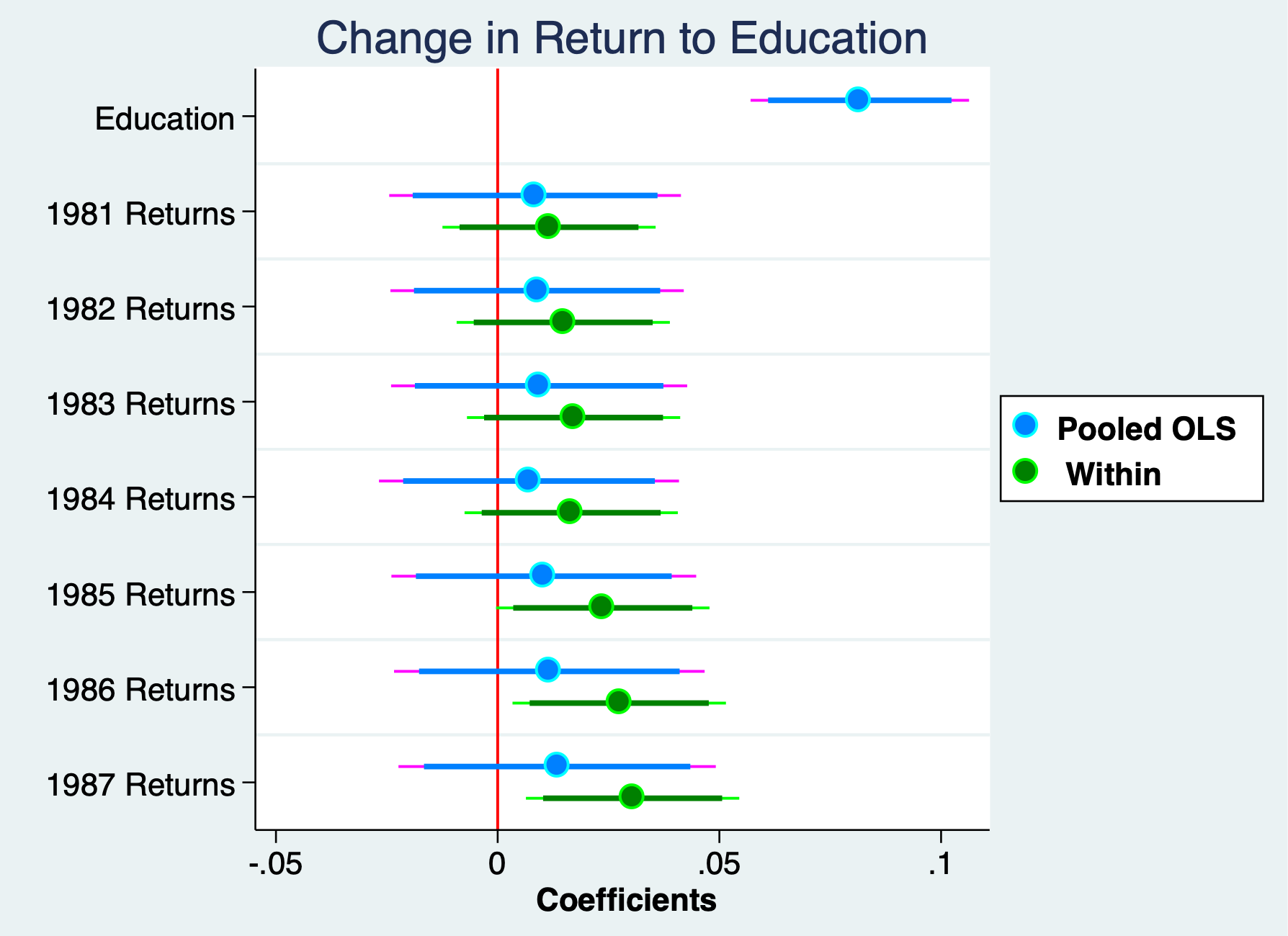
These are changes in the returns to education compared to the base year
of 1980 And only 1987xeducation and 1986xeducation appear to be
insignificant
. esttab OLS Within, mtitles se scalars(F r2) drop(0.d* 0.union 0.married)

────────────────────────────────────────────
                      (1)             (2)
                      OLS          Within
────────────────────────────────────────────
educ               0.0817***            0
                 (0.0126)             (.)

1.d81             -0.0357         -0.0224
                  (0.199)         (0.146)

1.d82             -0.0315        -0.00576
                  (0.200)         (0.146)

1.d83             -0.0343          0.0104
                  (0.201)         (0.146)

1.d84              0.0243          0.0844
                  (0.203)         (0.146)

1.d85             0.00588          0.0497
                  (0.205)         (0.146)

1.d86              0.0252          0.0656
                  (0.209)         (0.146)

1.d87              0.0373          0.0904
                  (0.215)         (0.146)

1.d81#c.educ      0.00844          0.0116
                 (0.0168)        (0.0123)

1.d82#c.educ      0.00889          0.0148
                 (0.0169)        (0.0123)

1.d83#c.educ      0.00935          0.0171
                 (0.0170)        (0.0123)

1.d84#c.educ      0.00707          0.0166
                 (0.0173)        (0.0123)

1.d85#c.educ       0.0104          0.0237
                 (0.0175)        (0.0123)

1.d86#c.educ       0.0117          0.0274*
                 (0.0179)        (0.0123)

1.d87#c.educ       0.0134          0.0304*
                 (0.0183)        (0.0123)

exper              0.0569***
                 (0.0154)

expersq          -0.00192*
               (0.000945)

1.married           0.123***       0.0548**
                 (0.0156)        (0.0184)

1.union             0.172***       0.0830***
                 (0.0171)        (0.0194)

_cons               0.218           1.362***
                  (0.164)        (0.0162)
────────────────────────────────────────────
N                    4360            4360
F                   50.92           48.91
r2                  0.182           0.171
────────────────────────────────────────────
Standard errors in parentheses
* p<0.05, ** p<0.01, *** p<0.001
Returns to education have increased by about 3.1% between 1987 and 1980.
. display (exp(0.0304)-1)*100
3.0866798
. quietly reg lwage c.edu##i.d8* exper expersq i.married i.union

. estimates store pooled

. quietly xtreg lwage c.edu##i.d8* i.married i.union, fe

. estimates store fe

. coefplot ///
>   (pooled, label("{bf:Pooled OLS}") mcolor(midblue) mlcolor(cyan) ///
>     ciopts(lcolor(magenta midblue))) /// options for first group
>   (fe, label("{bf: Within}") mcolor(green) mlcolor(lime) ///
>     ciopts(lcolor(lime green))), /// options for second gropu
>   title("Change in Return to Education") ///
>   keep(educ 1.d81#c.educ 1.d82#c.educ 1.d83#c.educ 1.d84#c.educ ///
>     1.d85#c.educ 1.d86#c.educ 1.d87#c.educ) ///
>   xline(0, lcolor(red) lwidth(medium)) scheme(jet_white) ///
>   xtitle("{bf: Coefficients}") ///
>   graphregion(margin(small)) ///
>   coeflabels(educ="Education" 1.d81#c.educ="1981 Returns" ///
>     1.d82#c.educ="1982 Returns" 1.d83#c.educ="1983 Returns" ///
>     1.d84#c.educ="1984 Returns" 1.d85#c.educ="1985 Returns" ///
>     1.d86#c.educ="1986 Returns" 1.d87#c.educ="1987 Returns") ///
>   msize(large) mcolor(%85) mlwidth(medium) msymbol(circle) /// marker options
>   levels(95 90) ciopts(lwidth(medthick thick) recast(rspike rcap)) ///ci options for all groups
>   legend(ring(1) col(1) pos(3) size(medsmall))
(note: scheme jet_white not found, using s2color)

. graph export "/Users/Sam/Desktop/Econ 645/Stata/week4_edu_returns.png", replace
(file /Users/Sam/Desktop/Econ 645/Stata/week4_edu_returns.png written in PNG format)
Test for Serial Correlation
. xtreg lwage c.edu##i.d8* i.married i.union, fe
note: educ omitted because of collinearity

Fixed-effects (within) regression               Number of obs     =      4,360
Group variable: nr                              Number of groups  =        545

R-sq:                                           Obs per group:
     within  = 0.1708                                         min =          8
     between = 0.1900                                         avg =        8.0
     overall = 0.1325                                         max =          8

                                                F(16,3799)        =      48.91
corr(u_i, Xb)  = 0.0991                         Prob > F          =     0.0000

─────────────┬────────────────────────────────────────────────────────────────
       lwage │      Coef.   Std. Err.      t    P>|t|     [95% Conf. Interval]
─────────────┼────────────────────────────────────────────────────────────────
        educ │          0  (omitted)
       1.d81 │  -.0224158   .1458885    -0.15   0.878    -.3084431    .2636114
       1.d82 │  -.0057611   .1458558    -0.04   0.968    -.2917243    .2802021
       1.d83 │   .0104297   .1458579     0.07   0.943    -.2755377    .2963971
       1.d84 │   .0843743   .1458518     0.58   0.563    -.2015811    .3703297
       1.d85 │   .0497253   .1458602     0.34   0.733    -.2362465    .3356971
       1.d86 │   .0656064   .1458917     0.45   0.653    -.2204273    .3516401
       1.d87 │   .0904448   .1458505     0.62   0.535     -.195508    .3763977
             │
  d81#c.educ │
          1  │   .0115854   .0122625     0.94   0.345    -.0124562    .0356271
             │
  d82#c.educ │
          1  │   .0147905   .0122635     1.21   0.228    -.0092533    .0388342
             │
  d83#c.educ │
          1  │   .0171182   .0122633     1.40   0.163    -.0069251    .0411615
             │
  d84#c.educ │
          1  │   .0165839   .0122657     1.35   0.176     -.007464    .0406319
             │
  d85#c.educ │
          1  │   .0237085   .0122738     1.93   0.053    -.0003554    .0477725
             │
  d86#c.educ │
          1  │   .0274123    .012274     2.23   0.026     .0033481    .0514765
             │
  d87#c.educ │
          1  │   .0304332   .0122723     2.48   0.013     .0063722    .0544942
             │
   1.married │   .0548205   .0184126     2.98   0.003      .018721      .09092
     1.union │   .0829785   .0194461     4.27   0.000     .0448527    .1211042
       _cons │   1.362459   .0162385    83.90   0.000     1.330622    1.394296
─────────────┼────────────────────────────────────────────────────────────────
     sigma_u │  .37264193
     sigma_e │  .35335713
         rho │  .52654439   (fraction of variance due to u_i)
─────────────┴────────────────────────────────────────────────────────────────
F test that all u_i=0: F(544, 3799) = 8.09                   Prob > F = 0.0000
predict u residuals
. predict u, resid
Our null hypothesis is that there is no serial correlation or the coefficient on our lagged residuals is zero. We’ll regress u on lag of u AR(1) model without a constant
. reg u l.u, noconst

      Source │       SS           df       MS      Number of obs   =     3,815
─────────────┼──────────────────────────────────   F(1, 3814)      =   2181.06
       Model │  332.737937         1  332.737937   Prob > F        =    0.0000
    Residual │  581.856111     3,814  .152557973   R-squared       =    0.3638
─────────────┼──────────────────────────────────   Adj R-squared   =    0.3636
       Total │  914.594048     3,815  .239736317   Root MSE        =    .39059

─────────────┬────────────────────────────────────────────────────────────────
           u │      Coef.   Std. Err.      t    P>|t|     [95% Conf. Interval]
─────────────┼────────────────────────────────────────────────────────────────
           u │
         L1. │   .5857228   .0125418    46.70   0.000     .5611336     .610312
─────────────┴────────────────────────────────────────────────────────────────
We can see that we have positive serial correlation since the coefficient on our lagged residual is positive and statistically significant. We will need to cluster our standard errors to account for the positive serial correlation.
If we use FE or FD, we cannot assess race, education, or experience since they remain constant, but we can include dummy interactions
Let’s test this for a wage gap between Black workers and non-Black workers. With Fixed Effects (Within) estimator we cannot estimate the wage gap, so we’ll use Pooled OLS. est clear
. eststo OLS: reg lwage c.edu##i.d8* i.black##i.d8* exper expersq i.married i.union
Source │ SS df MS Number of obs = 4,360
─────────────┼────────────────────────────────── F(27, 4332) = 37.78
Model │ 235.665339 27 8.72834589 Prob > F = 0.0000
Residual │ 1000.8643 4,332 .231039774 R-squared = 0.1906
─────────────┼────────────────────────────────── Adj R-squared = 0.1855
Total │ 1236.52964 4,359 .283672779 Root MSE = .48067
─────────────┬────────────────────────────────────────────────────────────────
lwage │ Coef. Std. Err. t P>|t| [95% Conf. Interval]
─────────────┼────────────────────────────────────────────────────────────────
educ │ .0830098 .0125217 6.63 0.000 .0584609 .1075588
1.d81 │ -.0412547 .1993287 -0.21 0.836 -.4320409 .3495315
1.d82 │ -.0152276 .1997638 -0.08 0.939 -.4068669 .3764117
1.d83 │ -.0268885 .2007155 -0.13 0.893 -.4203936 .3666166
1.d84 │ .0257253 .202407 0.13 0.899 -.371096 .4225465
1.d85 │ .0252159 .2050566 0.12 0.902 -.3768 .4272319
1.d86 │ .0228682 .2089636 0.11 0.913 -.3868074 .4325438
1.d87 │ .0552934 .2144675 0.26 0.797 -.3651726 .4757594
│
d81#c.educ │
1 │ .0083812 .0167209 0.50 0.616 -.0244003 .0411627
│
d82#c.educ │
1 │ .0080581 .0168149 0.48 0.632 -.0249077 .041024
│
d83#c.educ │
1 │ .0087321 .016972 0.51 0.607 -.0245417 .0420059
│
d84#c.educ │
1 │ .0065985 .0171926 0.38 0.701 -.0271079 .0403049
│
d85#c.educ │
1 │ .0091917 .0174659 0.53 0.599 -.0250503 .0434338
│
d86#c.educ │
1 │ .0109991 .0177943 0.62 0.537 -.0238868 .0458851
│
d87#c.educ │
1 │ .0119645 .0181818 0.66 0.511 -.0236811 .0476102
│
1.black │ -.0821357 .0645627 -1.27 0.203 -.2087116 .0444401
│
black#d81 │
1 1 │ .0350059 .0911407 0.38 0.701 -.1436765 .2136883
│
black#d82 │
1 1 │ -.0989736 .0911617 -1.09 0.278 -.2776971 .0797499
│
black#d83 │
1 1 │ -.0594933 .0911759 -0.65 0.514 -.2382447 .1192581
│
black#d84 │
1 1 │ -.0446436 .0911938 -0.49 0.624 -.2234302 .134143
│
black#d85 │
1 1 │ -.1412043 .0912107 -1.55 0.122 -.320024 .0376154
│
black#d86 │
1 1 │ -.0280978 .091229 -0.31 0.758 -.2069534 .1507578
│
black#d87 │
1 1 │ -.1448229 .0912847 -1.59 0.113 -.3237875 .0341418
│
exper │ .0616496 .0154296 4.00 0.000 .0313997 .0918995
expersq │ -.0020374 .0009435 -2.16 0.031 -.0038872 -.0001876
1.married │ .1069328 .0157148 6.80 0.000 .0761238 .1377419
1.union │ .1843211 .0171798 10.73 0.000 .15064 .2180023
_cons │ .1982792 .1638308 1.21 0.226 -.1229129 .5194713
─────────────┴────────────────────────────────────────────────────────────────
. eststo Within: xtreg lwage c.edu##i.d8* i.black##i.d8* i.married i.union, fe
note: educ omitted because of collinearity
note: 1.black omitted because of collinearity

Fixed-effects (within) regression               Number of obs     =      4,360
Group variable: nr                              Number of groups  =        545

R-sq:                                           Obs per group:
     within  = 0.1738                                         min =          8
     between = 0.1934                                         avg =        8.0
     overall = 0.1389                                         max =          8

                                                F(23,3792)        =      34.69
corr(u_i, Xb)  = 0.1049                         Prob > F          =     0.0000

─────────────┬────────────────────────────────────────────────────────────────
       lwage │      Coef.   Std. Err.      t    P>|t|     [95% Conf. Interval]
─────────────┼────────────────────────────────────────────────────────────────
        educ │          0  (omitted)
       1.d81 │  -.0276557   .1463492    -0.19   0.850    -.3145865    .2592752
       1.d82 │   .0162187   .1463125     0.11   0.912    -.2706402    .3030775
       1.d83 │   .0242781   .1463218     0.17   0.868     -.262599    .3111552
       1.d84 │   .0961124   .1463152     0.66   0.511    -.1907517    .3829765
       1.d85 │   .0806915   .1463169     0.55   0.581    -.2061759    .3675589
       1.d86 │    .075028   .1463527     0.51   0.608    -.2119097    .3619656
       1.d87 │   .1199805   .1463163     0.82   0.412    -.1668858    .4068467
             │
  d81#c.educ │
          1  │   .0117652   .0122599     0.96   0.337    -.0122714    .0358018
             │
  d82#c.educ │
          1  │   .0140603   .0122605     1.15   0.252    -.0099776    .0380982
             │
  d83#c.educ │
          1  │   .0166878   .0122603     1.36   0.174    -.0073497    .0407252
             │
  d84#c.educ │
          1  │   .0162498   .0122624     1.33   0.185    -.0077918    .0402914
             │
  d85#c.educ │
          1  │   .0227215   .0122702     1.85   0.064    -.0013353    .0467783
             │
  d86#c.educ │
          1  │    .027172   .0122704     2.21   0.027     .0031148    .0512291
             │
  d87#c.educ │
          1  │   .0295045   .0122688     2.40   0.016     .0054504    .0535587
             │
     1.black │          0  (omitted)
             │
   black#d81 │
        1 1  │   .0298494   .0669496     0.45   0.656    -.1014113    .1611101
             │
   black#d82 │
        1 1  │  -.1111954   .0669827    -1.66   0.097     -.242521    .0201302
             │
   black#d83 │
        1 1  │  -.0687691   .0669927    -1.03   0.305    -.2001144    .0625761
             │
   black#d84 │
        1 1  │  -.0589417   .0670094    -0.88   0.379    -.1903196    .0724362
             │
   black#d85 │
        1 1  │  -.1573439   .0670161    -2.35   0.019     -.288735   -.0259527
             │
   black#d86 │
        1 1  │  -.0458512   .0670197    -0.68   0.494    -.1772493    .0855469
             │
   black#d87 │
        1 1  │  -.1494466    .067063    -2.23   0.026    -.2809297   -.0179636
             │
   1.married │   .0516758   .0184369     2.80   0.005     .0155286    .0878229
     1.union │   .0845706    .019456     4.35   0.000     .0464254    .1227157
       _cons │   1.362641   .0162264    83.98   0.000     1.330828    1.394455
─────────────┼────────────────────────────────────────────────────────────────
     sigma_u │  .37090778
     sigma_e │  .35303669
         rho │   .5246707   (fraction of variance due to u_i)
─────────────┴────────────────────────────────────────────────────────────────
F test that all u_i=0: F(544, 3792) = 8.01                   Prob > F = 0.0000
. esttab OLS Within, mtitles se scalars(F r2) drop(0.d* 0.b* 1.black#0.d* 0.union 0.married)

────────────────────────────────────────────
                      (1)             (2)
                      OLS          Within
────────────────────────────────────────────
educ               0.0830***            0
                 (0.0125)             (.)

1.d81             -0.0413         -0.0277
                  (0.199)         (0.146)

1.d82             -0.0152          0.0162
                  (0.200)         (0.146)

1.d83             -0.0269          0.0243
                  (0.201)         (0.146)

1.d84              0.0257          0.0961
                  (0.202)         (0.146)

1.d85              0.0252          0.0807
                  (0.205)         (0.146)

1.d86              0.0229          0.0750
                  (0.209)         (0.146)

1.d87              0.0553           0.120
                  (0.214)         (0.146)

1.d81#c.educ      0.00838          0.0118
                 (0.0167)        (0.0123)

1.d82#c.educ      0.00806          0.0141
                 (0.0168)        (0.0123)

1.d83#c.educ      0.00873          0.0167
                 (0.0170)        (0.0123)

1.d84#c.educ      0.00660          0.0162
                 (0.0172)        (0.0123)

1.d85#c.educ      0.00919          0.0227
                 (0.0175)        (0.0123)

1.d86#c.educ       0.0110          0.0272*
                 (0.0178)        (0.0123)

1.d87#c.educ       0.0120          0.0295*
                 (0.0182)        (0.0123)

1.black           -0.0821               0
                 (0.0646)             (.)

1.black#1~81       0.0350          0.0298
                 (0.0911)        (0.0669)

1.black#1~82      -0.0990          -0.111
                 (0.0912)        (0.0670)

1.black#1~83      -0.0595         -0.0688
                 (0.0912)        (0.0670)

1.black#1~84      -0.0446         -0.0589
                 (0.0912)        (0.0670)

1.black#1~85       -0.141          -0.157*
                 (0.0912)        (0.0670)

1.black#1~86      -0.0281         -0.0459
                 (0.0912)        (0.0670)

1.black#1~87       -0.145          -0.149*
                 (0.0913)        (0.0671)

exper              0.0616***
                 (0.0154)

expersq          -0.00204*
               (0.000944)

1.married           0.107***       0.0517**
                 (0.0157)        (0.0184)

1.union             0.184***       0.0846***
                 (0.0172)        (0.0195)

_cons               0.198           1.363***
                  (0.164)        (0.0162)
────────────────────────────────────────────
N                    4360            4360
F                   37.78           34.69
r2                  0.191           0.174
────────────────────────────────────────────
Standard errors in parentheses
* p<0.05, ** p<0.01, *** p<0.001
We’ll use three methods to estimate the returns to marriage for men: Pooled OLS, Fixed Effects (Within), and Random Effects. We cannot estimate the coefficients for Black and Latino/Latina.
. use "wagepan.dta", clear
We can use the wagepan data again to estimate the returns to marriage for men. We will compare the Pooled OLS, FE (Within), and Random Effects estimates
Set Panel
. xtset nr year
       panel variable:  nr (strongly balanced)
        time variable:  year, 1980 to 1987
                delta:  1 unit
. reg lwage educ i.black i.hisp exper expersq married union i.d8*

      Source │       SS           df       MS      Number of obs   =     4,360
─────────────┼──────────────────────────────────   F(14, 4345)     =     72.46
       Model │  234.048277        14  16.7177341   Prob > F        =    0.0000
    Residual │  1002.48136     4,345  .230720682   R-squared       =    0.1893
─────────────┼──────────────────────────────────   Adj R-squared   =    0.1867
       Total │  1236.52964     4,359  .283672779   Root MSE        =    .48033

─────────────┬────────────────────────────────────────────────────────────────
       lwage │      Coef.   Std. Err.      t    P>|t|     [95% Conf. Interval]
─────────────┼────────────────────────────────────────────────────────────────
        educ │   .0913498   .0052374    17.44   0.000     .0810819    .1016177
     1.black │  -.1392342   .0235796    -5.90   0.000    -.1854622   -.0930062
      1.hisp │   .0160195   .0207971     0.77   0.441    -.0247535    .0567925
       exper │   .0672345   .0136948     4.91   0.000     .0403856    .0940834
     expersq │  -.0024117     .00082    -2.94   0.003    -.0040192   -.0008042
     married │   .1082529   .0156894     6.90   0.000     .0774937    .1390122
       union │   .1824613   .0171568    10.63   0.000     .1488253    .2160973
       1.d81 │     .05832   .0303536     1.92   0.055    -.0011886    .1178286
       1.d82 │   .0627744   .0332141     1.89   0.059    -.0023421    .1278909
       1.d83 │   .0620117   .0366601     1.69   0.091    -.0098608    .1338843
       1.d84 │   .0904672   .0400907     2.26   0.024      .011869    .1690654
       1.d85 │   .1092463   .0433525     2.52   0.012     .0242533    .1942393
       1.d86 │   .1419596    .046423     3.06   0.002     .0509469    .2329723
       1.d87 │   .1738334    .049433     3.52   0.000     .0769194    .2707474
       _cons │   .0920558   .0782701     1.18   0.240    -.0613935    .2455051
─────────────┴────────────────────────────────────────────────────────────────

. eststo m1: quietly reg lwage educ i.black i.hisp exper expersq married union i.d8*
The Pooled OLS data are likley upward biased - self-selection into marriage and we will have positive serial correlation so we really should cluster our standard errors by the group id.
. xtreg lwage educ i.black i.hisp exper expersq married union i.d8*, fe
note: educ omitted because of collinearity
note: 1.black omitted because of collinearity
note: 1.hisp omitted because of collinearity
note: 1.d87 omitted because of collinearity

Fixed-effects (within) regression               Number of obs     =      4,360
Group variable: nr                              Number of groups  =        545

R-sq:                                           Obs per group:
     within  = 0.1806                                         min =          8
     between = 0.0005                                         avg =        8.0
     overall = 0.0635                                         max =          8

                                                F(10,3805)        =      83.85
corr(u_i, Xb)  = -0.1212                        Prob > F          =     0.0000

─────────────┬────────────────────────────────────────────────────────────────
       lwage │      Coef.   Std. Err.      t    P>|t|     [95% Conf. Interval]
─────────────┼────────────────────────────────────────────────────────────────
        educ │          0  (omitted)
     1.black │          0  (omitted)
      1.hisp │          0  (omitted)
       exper │   .1321464   .0098247    13.45   0.000     .1128842    .1514087
     expersq │  -.0051855   .0007044    -7.36   0.000    -.0065666   -.0038044
     married │   .0466804   .0183104     2.55   0.011     .0107811    .0825796
       union │   .0800019   .0193103     4.14   0.000     .0421423    .1178614
       1.d81 │   .0190448   .0203626     0.94   0.350    -.0208779    .0589674
       1.d82 │   -.011322   .0202275    -0.56   0.576    -.0509798    .0283359
       1.d83 │  -.0419955   .0203205    -2.07   0.039    -.0818357   -.0021553
       1.d84 │  -.0384709   .0203144    -1.89   0.058    -.0782991    .0013573
       1.d85 │  -.0432498   .0202458    -2.14   0.033    -.0829434   -.0035562
       1.d86 │  -.0273819   .0203863    -1.34   0.179    -.0673511    .0125872
       1.d87 │          0  (omitted)
       _cons │    1.02764   .0299499    34.31   0.000     .9689201    1.086359
─────────────┼────────────────────────────────────────────────────────────────
     sigma_u │   .4009279
     sigma_e │  .35099001
         rho │  .56612236   (fraction of variance due to u_i)
─────────────┴────────────────────────────────────────────────────────────────
F test that all u_i=0: F(544, 3805) = 9.64                   Prob > F = 0.0000
We use estimates store to store our FE (Within) estimates to compare
. estimates store femodel

. eststo m2: quietly xtreg lwage educ i.black i.hisp exper expersq married union i.d8*, fe
We can use the theta option to find the lambda-hat GLS transformaton https://www.stata.com/manuals/xtxtreg.pdf
. xtreg lwage educ i.black i.hisp exper expersq married union i.d8*, re theta

Random-effects GLS regression                   Number of obs     =      4,360
Group variable: nr                              Number of groups  =        545

R-sq:                                           Obs per group:
     within  = 0.1799                                         min =          8
     between = 0.1860                                         avg =        8.0
     overall = 0.1830                                         max =          8

                                                Wald chi2(14)     =     957.77
corr(u_i, X)   = 0 (assumed)                    Prob > chi2       =     0.0000
theta          = .64291089

─────────────┬────────────────────────────────────────────────────────────────
       lwage │      Coef.   Std. Err.      z    P>|z|     [95% Conf. Interval]
─────────────┼────────────────────────────────────────────────────────────────
        educ │   .0918763   .0106597     8.62   0.000     .0709836    .1127689
     1.black │  -.1393767   .0477228    -2.92   0.003    -.2329117   -.0458417
      1.hisp │   .0217317   .0426063     0.51   0.610    -.0617751    .1052385
       exper │   .1057545   .0153668     6.88   0.000     .0756361    .1358729
     expersq │  -.0047239   .0006895    -6.85   0.000    -.0060753   -.0033726
     married │    .063986   .0167742     3.81   0.000     .0311091    .0968629
       union │   .1061344   .0178539     5.94   0.000     .0711415    .1411273
       1.d81 │    .040462   .0246946     1.64   0.101    -.0079385    .0888626
       1.d82 │   .0309212   .0323416     0.96   0.339    -.0324672    .0943096
       1.d83 │   .0202806    .041582     0.49   0.626    -.0612186    .1017798
       1.d84 │   .0431187   .0513163     0.84   0.401    -.0574595    .1436969
       1.d85 │   .0578155   .0612323     0.94   0.345    -.0621977    .1778286
       1.d86 │   .0919476   .0712293     1.29   0.197    -.0476592    .2315544
       1.d87 │   .1349289   .0813135     1.66   0.097    -.0244427    .2943005
       _cons │   .0235864   .1506683     0.16   0.876     -.271718    .3188907
─────────────┼────────────────────────────────────────────────────────────────
     sigma_u │  .32460315
     sigma_e │  .35099001
         rho │  .46100216   (fraction of variance due to u_i)
─────────────┴────────────────────────────────────────────────────────────────

. eststo m3: quietly xtreg lwage educ i.black i.hisp exper expersq married union i.d8*, re
Our lambda-hat is 0.643, which means it is closer to the FE estimator than the Pooled OLS estimator.
. hausman femodel ., sigmamore

Note: the rank of the differenced variance matrix (5) does not equal the number of coefficients being tested
        (10); be sure this is what you expect, or there may be problems computing the test.  Examine the output
        of your estimators for anything unexpected and possibly consider scaling your variables so that the
        coefficients are on a similar scale.

                 ──── Coefficients ────
             │      (b)          (B)            (b-B)     sqrt(diag(V_b-V_B))
             │    femodel         m3         Difference          S.E.
─────────────┼────────────────────────────────────────────────────────────────
       exper │    .1321464     .1057545        .0263919               .
     expersq │   -.0051855    -.0047239       -.0004616        .0001533
     married │    .0466804      .063986       -.0173057        .0074632
       union │    .0800019     .1061344       -.0261326        .0074922
       1.d81 │    .0190448      .040462       -.0214172               .
       1.d82 │    -.011322     .0309212       -.0422431               .
       1.d83 │   -.0419955     .0202806       -.0622762               .
       1.d84 │   -.0384709     .0431187       -.0815896               .
       1.d85 │   -.0432498     .0578155       -.1010653               .
       1.d86 │   -.0273819     .0919476       -.1193295               .
─────────────┴────────────────────────────────────────────────────────────────
                           b = consistent under Ho and Ha; obtained from xtreg
            B = inconsistent under Ha, efficient under Ho; obtained from xtreg

    Test:  Ho:  difference in coefficients not systematic

                  chi2(5) = (b-B)'[(V_b-V_B)^(-1)](b-B)
                          =       26.22
                Prob>chi2 =      0.0001
                (V_b-V_B is not positive definite)
We reject the null hypothesis and a_i is correlated with the explanatory variables - We reject the Random Effects Model
. esttab m1 m2 m3, drop(0.black 0.hisp 0.d8*) mtitles("Pooled OLS" "Within Model" "RE Model")

────────────────────────────────────────────────────────────
                      (1)             (2)             (3)
               Pooled OLS    Within Model        RE Model
────────────────────────────────────────────────────────────
educ               0.0913***            0          0.0919***
                  (17.44)             (.)          (8.62)

1.black            -0.139***            0          -0.139**
                  (-5.90)             (.)         (-2.92)

1.hisp             0.0160               0          0.0217
                   (0.77)             (.)          (0.51)

exper              0.0672***        0.132***        0.106***
                   (4.91)         (13.45)          (6.88)

expersq          -0.00241**      -0.00519***     -0.00472***
                  (-2.94)         (-7.36)         (-6.85)

married             0.108***       0.0467*         0.0640***
                   (6.90)          (2.55)          (3.81)

union               0.182***       0.0800***        0.106***
                  (10.63)          (4.14)          (5.94)

1.d81              0.0583          0.0190          0.0405
                   (1.92)          (0.94)          (1.64)

1.d82              0.0628         -0.0113          0.0309
                   (1.89)         (-0.56)          (0.96)

1.d83              0.0620         -0.0420*         0.0203
                   (1.69)         (-2.07)          (0.49)

1.d84              0.0905*        -0.0385          0.0431
                   (2.26)         (-1.89)          (0.84)

1.d85               0.109*        -0.0432*         0.0578
                   (2.52)         (-2.14)          (0.94)

1.d86               0.142**       -0.0274          0.0919
                   (3.06)         (-1.34)          (1.29)

1.d87               0.174***            0           0.135
                   (3.52)             (.)          (1.66)

_cons              0.0921           1.028***       0.0236
                   (1.18)         (34.31)          (0.16)
────────────────────────────────────────────────────────────
N                    4360            4360            4360
────────────────────────────────────────────────────────────
t statistics in parentheses
* p<0.05, ** p<0.01, *** p<0.001
. display (exp(.108)-1)*100
11.404775

. display (exp(.0467)-1)*100
4.780762

. display (exp(.064)-1)*100
6.6092399
We can see that the marriage premium falls from 11.4% in Pooled OLS to 4.8% in Fixed Effects. If we didn’t reject our RE model, it would have been 6.6%.
The difference between the 11.4% Pooled OLS and the 4.8% in the Within Model might comes from self-selection in marriage (they would have made more money even if they weren’t married), and employers paying married men more if marriage is a sign of stability. But, we cannot distinguish these two hypothesis with this research design.
. quietly reg lwage educ i.black i.hisp exper expersq married union i.d8*

. estimates store pooled

. quietly xtreg lwage educ i.black i.hisp exper expersq married union i.d8*, fe

. estimates store fe

. quietly xtreg lwage educ i.black i.hisp exper expersq married union i.d8*, re theta

. estimates store re

. coefplot ///
> (pooled, label("{bf:Pooled OLS}") mcolor(midblue) mlcolor(cyan) ///
>   ciopts(lcolor(magenta midblue))) /// options for first group
> (fe, label("{bf: Within}") mcolor(green) mlcolor(lime) ///
>   ciopts(lcolor(lime green))) /// options for second group
> (re, label("{bf: Random Effects}") mcolor(yellow) mlcolor(gold) ///
>   ciopts(lcolor(gold yellow))), /// options for third group
>   title("Returns to Marriage for Men") ///
>   keep(married) ///
>   xline(0, lcolor(red) lpattern(dash) lwidth(medium)) scheme(jet_white) ///
>   xtitle("{bf: Coefficients}") ///
>   graphregion(margin(small)) ///
>   coeflabels(married="Married") ///
>   msize(large) mcolor(%85) mlwidth(medium) msymbol(circle) /// marker options
>   levels(95 90) ciopts(lwidth(medthick thick) recast(rspike rcap)) ///ci options for all groups
>   legend(ring(1) col(1) pos(3) size(medsmall))
(note: scheme jet_white not found, using s2color)

. graph export "/Users/Sam/Desktop/Econ 645/Stata/week4_married_returns.png", replace
(file /Users/Sam/Desktop/Econ 645/Stata/week4_married_returns.png written in PNG format)

Exercise 1:
. use "rental.dta", clear
The data on rental prices and other variables in college towns from 1980 to 1990. Do more students affect the prices? The general model with unobserved fixed effects is ln(rent)=b0+d0y90+b1ln(pop)+b2ln(avginc)+b3pctstu+a_i+u_i Where pop is city population, avginc is average income, pctstu is the student percent of the population, and rent is the nominal rental prices
Estimate a Pooled OLS. What does the estimate on y90 tell you?
Are there concerns with the standard errors in the Pooled OLS?
Use a First difference model. Does the coefficient on b3 change?
Use a FE Within model. Are the results the same as the FD model?
. xtset city year, delta(10)
       panel variable:  city (strongly balanced)
        time variable:  year, 80 to 90
                delta:  10 units
. reg lrent i.y90 lpop lavginc pctstu, robust

Linear regression                               Number of obs     =        128
                                                F(4, 123)         =     223.26
                                                Prob > F          =     0.0000
                                                R-squared         =     0.8613
                                                Root MSE          =     .12592

─────────────┬────────────────────────────────────────────────────────────────
             │               Robust
       lrent │      Coef.   Std. Err.      t    P>|t|     [95% Conf. Interval]
─────────────┼────────────────────────────────────────────────────────────────
       1.y90 │   .2622267   .0579584     4.52   0.000     .1475017    .3769517
        lpop │   .0406863   .0223732     1.82   0.071       -.0036    .0849726
     lavginc │   .5714461   .0989016     5.78   0.000     .3756765    .7672157
      pctstu │   .0050436   .0011488     4.39   0.000     .0027696    .0073176
       _cons │  -.5688069   .8506229    -0.67   0.505    -2.252563    1.114949
─────────────┴────────────────────────────────────────────────────────────────
. reg d.lrent i.y90 d.lpop d.lavginc d.pctstu
note: 1.y90 omitted because of collinearity

      Source │       SS           df       MS      Number of obs   =        64
─────────────┼──────────────────────────────────   F(3, 60)        =      9.51
       Model │  .231738668         3  .077246223   Prob > F        =    0.0000
    Residual │  .487362198        60  .008122703   R-squared       =    0.3223
─────────────┼──────────────────────────────────   Adj R-squared   =    0.2884
       Total │  .719100867        63  .011414299   Root MSE        =    .09013

─────────────┬────────────────────────────────────────────────────────────────
     D.lrent │      Coef.   Std. Err.      t    P>|t|     [95% Conf. Interval]
─────────────┼────────────────────────────────────────────────────────────────
       1.y90 │          0  (omitted)
             │
        lpop │
         D1. │   .0722456   .0883426     0.82   0.417     -.104466    .2489571
             │
     lavginc │
         D1. │   .3099605   .0664771     4.66   0.000     .1769865    .4429346
             │
      pctstu │
         D1. │   .0112033   .0041319     2.71   0.009     .0029382    .0194684
             │
       _cons │   .3855214   .0368245    10.47   0.000     .3118615    .4591813
─────────────┴────────────────────────────────────────────────────────────────
. xtreg lrent i.y90 lpop lavginc pctstu, fe

Fixed-effects (within) regression               Number of obs     =        128
Group variable: city                            Number of groups  =         64

R-sq:                                           Obs per group:
     within  = 0.9765                                         min =          2
     between = 0.2173                                         avg =        2.0
     overall = 0.7597                                         max =          2

                                                F(4,60)           =     624.15
corr(u_i, Xb)  = -0.1297                        Prob > F          =     0.0000

─────────────┬────────────────────────────────────────────────────────────────
       lrent │      Coef.   Std. Err.      t    P>|t|     [95% Conf. Interval]
─────────────┼────────────────────────────────────────────────────────────────
       1.y90 │   .3855214   .0368245    10.47   0.000     .3118615    .4591813
        lpop │   .0722456   .0883426     0.82   0.417     -.104466    .2489571
     lavginc │   .3099605   .0664771     4.66   0.000     .1769865    .4429346
      pctstu │   .0112033   .0041319     2.71   0.009     .0029382    .0194684
       _cons │   1.409384   1.167238     1.21   0.232    -.9254394    3.744208
─────────────┼────────────────────────────────────────────────────────────────
     sigma_u │  .15905877
     sigma_e │  .06372873
         rho │   .8616755   (fraction of variance due to u_i)
─────────────┴────────────────────────────────────────────────────────────────
F test that all u_i=0: F(63, 60) = 6.67                      Prob > F = 0.0000
Exercise 2:
. use "airfare.dta", clear
We will assess concentration of airline on airfare. Our model: ln(fare) = b0 + b1concen + b2ln(dist) + b3*(ln(dist))^2 + a_i + u_i
Estimate the Pooled OLS with time binaries
. reg lfare concen ldist ldistsq i.y99 i.y00

      Source │       SS           df       MS      Number of obs   =     4,596
─────────────┼──────────────────────────────────   F(5, 4590)      =    627.18
       Model │  355.197587         5  71.0395174   Prob > F        =    0.0000
    Residual │  519.896787     4,590  .113267274   R-squared       =    0.4059
─────────────┼──────────────────────────────────   Adj R-squared   =    0.4052
       Total │  875.094374     4,595  .190444913   Root MSE        =    .33655

─────────────┬────────────────────────────────────────────────────────────────
       lfare │      Coef.   Std. Err.      t    P>|t|     [95% Conf. Interval]
─────────────┼────────────────────────────────────────────────────────────────
      concen │   .3609856   .0300677    12.01   0.000     .3020384    .4199327
       ldist │  -.9018838   .1282905    -7.03   0.000    -1.153395   -.6503727
     ldistsq │   .1030514   .0097268    10.59   0.000     .0839822    .1221207
       1.y99 │   .0272979   .0121656     2.24   0.025     .0034475    .0511483
       1.y00 │   .0893211    .012169     7.34   0.000     .0654641    .1131782
       _cons │   6.219743   .4206248    14.79   0.000     5.395116     7.04437
─────────────┴────────────────────────────────────────────────────────────────
What does a change in concen of 10 for airfare?
. sum concen

    Variable │        Obs        Mean    Std. Dev.       Min        Max
─────────────┼─────────────────────────────────────────────────────────
      concen │      4,596    .6101149     .196435      .1605          1
What does the quadratic on distance mean Decreasing at a increasing rate - use quadratic formula for when distance on airfare is 0 Set Panel
. xtset id year
       panel variable:  id (strongly balanced)
        time variable:  year, 1997 to 2000
                delta:  1 unit
Estimate a RE model
. xtreg lfare concen ldist ldistsq i.y99 i.y00, re theta

Random-effects GLS regression                   Number of obs     =      4,596
Group variable: id                              Number of groups  =      1,149

R-sq:                                           Obs per group:
     within  = 0.1282                                         min =          4
     between = 0.4179                                         avg =        4.0
     overall = 0.4030                                         max =          4

                                                Wald chi2(5)      =    1331.49
corr(u_i, X)   = 0 (assumed)                    Prob > chi2       =     0.0000
theta          = .83489895

─────────────┬────────────────────────────────────────────────────────────────
       lfare │      Coef.   Std. Err.      z    P>|z|     [95% Conf. Interval]
─────────────┼────────────────────────────────────────────────────────────────
      concen │    .216343   .0265686     8.14   0.000     .1642694    .2684166
       ldist │  -.8544998   .2464622    -3.47   0.001    -1.337557   -.3714428
     ldistsq │   .0977308   .0186343     5.24   0.000     .0612083    .1342532
       1.y99 │   .0255419   .0038794     6.58   0.000     .0179385    .0331454
       1.y00 │   .0870883   .0038876    22.40   0.000     .0794686    .0947079
       _cons │   6.232589   .8098919     7.70   0.000      4.64523    7.819948
─────────────┼────────────────────────────────────────────────────────────────
     sigma_u │  .31930578
     sigma_e │   .1069025
         rho │  .89920879   (fraction of variance due to u_i)
─────────────┴────────────────────────────────────────────────────────────────
Estimate a FE model
. xtreg lfare concen ldist ldistsq i.y99 i.y00, fe
note: ldist omitted because of collinearity
note: ldistsq omitted because of collinearity

Fixed-effects (within) regression               Number of obs     =      4,596
Group variable: id                              Number of groups  =      1,149

R-sq:                                           Obs per group:
     within  = 0.1286                                         min =          4
     between = 0.0576                                         avg =        4.0
     overall = 0.0102                                         max =          4

                                                F(3,3444)         =     169.47
corr(u_i, Xb)  = -0.2143                        Prob > F          =     0.0000

─────────────┬────────────────────────────────────────────────────────────────
       lfare │      Coef.   Std. Err.      t    P>|t|     [95% Conf. Interval]
─────────────┼────────────────────────────────────────────────────────────────
      concen │    .177761   .0294665     6.03   0.000     .1199873    .2355346
       ldist │          0  (omitted)
     ldistsq │          0  (omitted)
       1.y99 │   .0250736   .0038791     6.46   0.000      .017468    .0326791
       1.y00 │   .0864927   .0038892    22.24   0.000     .0788673    .0941181
       _cons │   4.959254   .0183174   270.74   0.000      4.92334    4.995168
─────────────┼────────────────────────────────────────────────────────────────
     sigma_u │  .43441394
     sigma_e │   .1069025
         rho │  .94290028   (fraction of variance due to u_i)
─────────────┴────────────────────────────────────────────────────────────────
F test that all u_i=0: F(1148, 3444) = 60.09                 Prob > F = 0.0000
Generate and replace will be the workhorses of creating and modifying variables We’ll deal with generating binary variables We’ll look into missing data and how to handle it Note: Please do not label your missing data, it just is a pain to deal with later Egen is also a very practical and useful command (I wish other software packages had this feature that is so easy to implement We’ll deal with strings and converting between numerics and strings We’ll also work with rename
One of the most basic tasks is to create, replace, and modify variables. Stata provides some nice and easy commands to work with variable generation and modification relative to other statistical software packages.
The generate command and replace command will be important, but Stata has a very helpful command called egen. It can be used to create new variables from old variables, especially when working with groups of observations. Egen becomes even more helpful when it is combined with bysort. We can sort our group and find the max, min, sum, etc. of a group of observations, which can come in handy when we are working with panel data
Futhermore, using indexes can make our generation commands more useful for creating lags or rebasing our data.
Set our working directory
. cd "/Users/Sam/Desktop/Econ 645/Data/Mitchell"
/Users/Sam/Desktop/Econ 645/Data/Mitchell
Let’s get our data
. use wws, clear
(Working Women Survey)
The generate command is one that you have plenty of experience with already, but there are some helpful tips when working with generate. What we’ll do first is to create a new variable called weekly wages. This will be based off of hourly wages and hours at work by women.
Let’s look at hourly wages for women
. summarize wage

    Variable │        Obs        Mean    Std. Dev.       Min        Max
─────────────┼─────────────────────────────────────────────────────────
        wage │      2,246    288.2885    9595.692          0     380000
Look for outliers
. list id wage if wage > 1000

      ┌─────────────────┐
      │ idcode     wage │
      ├─────────────────┤
 893. │   3145   380000 │
1241. │   2341   250000 │
      └─────────────────┘
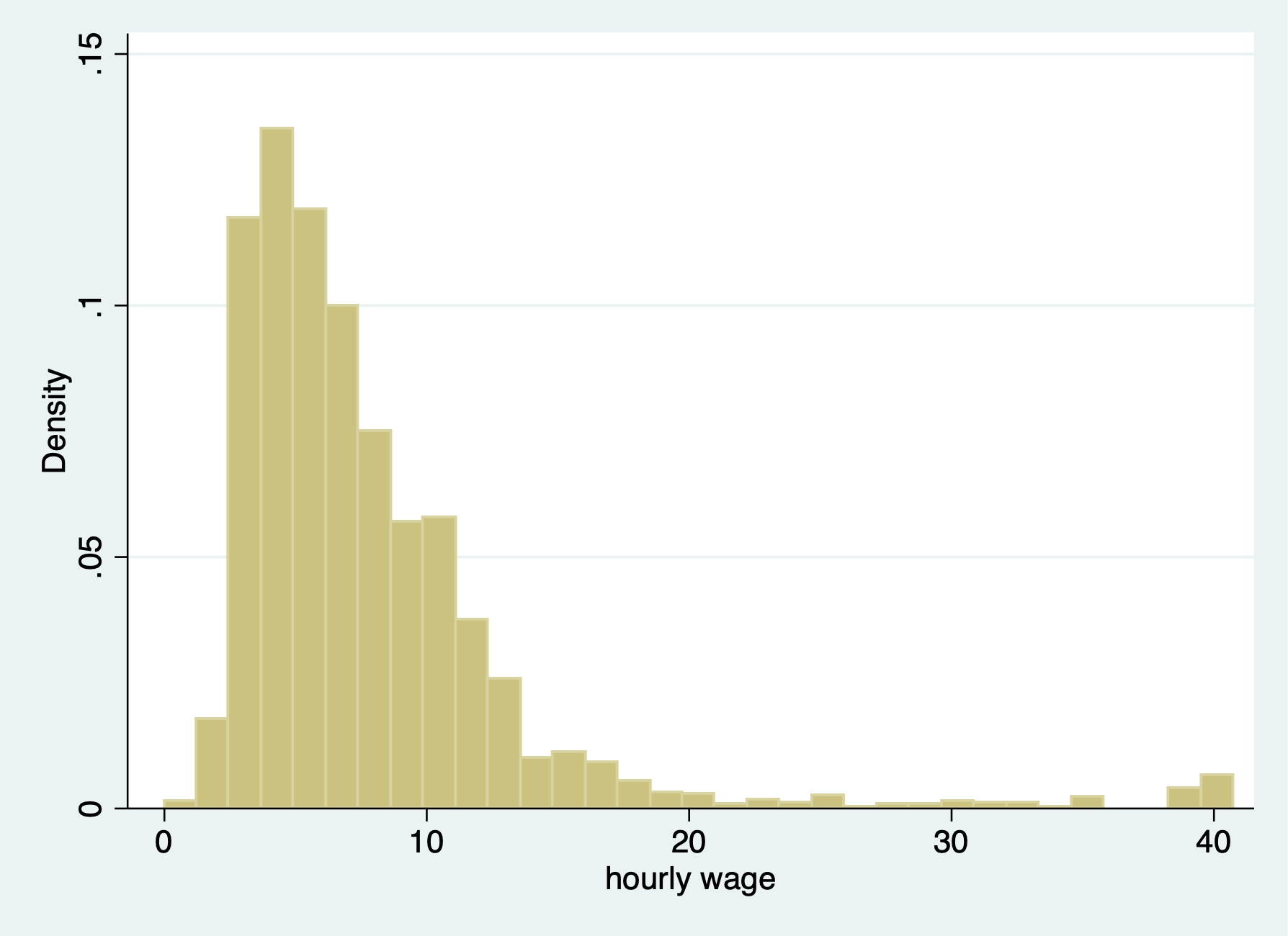
A histogram is helpful too
. histogram wage if wage < 1000
(bin=33, start=0, width=1.2347451)

. graph export "/Users/Sam/Desktop/Econ 645/Stata/week4_wages_hist.png", replace
(file /Users/Sam/Desktop/Econ 645/Stata/week4_wages_hist.png written in PNG format)
Let’s look at hours
. summarize hours

    Variable │        Obs        Mean    Std. Dev.       Min        Max
─────────────┼─────────────────────────────────────────────────────────
       hours │      2,242    37.21811    10.50914          1         80
Let’s look at histogram of hours
. histogram hours
(bin=33, start=1, width=2.3939394)
Let’s create our weekly wages
. gen weekwage = wage*hours
(4 missing values generated)
We’ll summarize our new variable
. summarize weekwage, detail

                          weekwage
─────────────────────────────────────────────────────────────
      Percentiles      Smallest
 1%     18.01074              0
 5%     61.99676        4.64573
10%     85.02411       6.038647       Obs               2,242
25%     146.3211        8.05153       Sum of Wgt.       2,242

50%      241.401                      Mean           11539.95
                        Largest       Std. Dev.      384170.1
75%     385.5072       1607.924
90%     526.4493           1920       Variance       1.48e+11
95%      681.159       1.00e+07       Skewness       35.42672
99%     1607.923       1.52e+07       Kurtosis       1294.728
We need to find our oultiers
. list id weekwage if weekwage > 80000

      ┌───────────────────┐
      │ idcode   weekwage │
      ├───────────────────┤
  19. │   5111          . │
 372. │   4324          . │
 804. │   3318          . │
 893. │   3145   15200000 │
1139. │   2583          . │
      ├───────────────────┤
1241. │   2341   10000000 │
      └───────────────────┘
Notice! Our missing values were captured in our outlier check! Why? Because missing values are considered very large values. This is important because when creating binary or categorical variables through qualifiers, make sure you top code your qualifiers For example, if we are creating a binary on part-time vs full-time We need to top code so we don’t count missing hours as full-time workers, such as hours > 35 & hours < 999999, or, hours > 35 & !missing(hours), оr else you may categorize missing hours as full-time.
Let’s plot our weekly wages
. histogram weekwage if weekwage < 80000
(bin=33, start=0, width=58.181818)
Another helpful trick is the before and after options It might be helpful to have the newly created variable next to a similar variable, so let’s drop our variable and generate it again with the after option
. drop weekwage
. gen weekwage = wage*hours, after(wage)
(4 missing values generated)
We use our replace command to modify a variable that has already been created. Similar to generate, you probably already have experience with replace, but we’ll go over some useful tips.
Let’s look at married and nevermarried variables
. tabulate married nevermarried

           │   Woman never been
           │        married
   married │         0          1 │     Total
───────────┼──────────────────────┼──────────
         0 │       570        234 │       804
         1 │     1,440          2 │     1,442
───────────┼──────────────────────┼──────────
     Total │     2,010        236 │     2,246
We’ll create a categorical variable called maritalstatus.
. gen maritalstatus = .
(2,246 missing values generated)
I recommend generating a new categorical variable as missing instead of zero, because this prevents missing variables from being categorized as 0.
We generally use qualifers “=, >, <, >=, <=, !” when working with replace Let’s replace the marital status variable with married and nevermarried as qualifiers
. replace maritalstatus = 1 if married==0 & nevermarried==1
(234 real changes made)

. replace maritalstatus = 2 if married==1 & nevermarried==0
(1,440 real changes made)

. replace maritalstatus = 3 if married==0 & nevermarried==0
(570 real changes made)
It’s always a good idea to double check the varilabes against the variables they were created from to make sure your categories are what they are supposed to be
. tabulate maritalstatus

maritalstat │
         us │      Freq.     Percent        Cum.
────────────┼───────────────────────────────────
          1 │        234       10.43       10.43
          2 │      1,440       64.17       74.60
          3 │        570       25.40      100.00
────────────┼───────────────────────────────────
      Total │      2,244      100.00

. table maritalstatus married nevermarried

──────────┬─────────────────────────────
          │ Woman never been married and
          │           married
maritalst │ ───── 0 ────    ───── 1 ────
atus      │     0      1        0      1
──────────┼─────────────────────────────
        1 │                   234
        2 │        1,440
        3 │   570
──────────┴─────────────────────────────
Let’s label our values similar to last week Labeling is a good practice for your future self or for others replicating
. label define maritalstatus1 1 "Single" 2 "Married" 3 "Divorced or Widowed"

. label values maritalstatus maritalstatus1

. label variable maritalstatus "Marital Status"

. tabulate maritalstatus

     Marital Status │      Freq.     Percent        Cum.
────────────────────┼───────────────────────────────────
             Single │        234       10.43       10.43
            Married │      1,440       64.17       74.60
Divorced or Widowed │        570       25.40      100.00
────────────────────┼───────────────────────────────────
              Total │      2,244      100.00
Let’s create a new varible called over40hours which will be categorized as 1 if it is over 40 hours, and 0 if it is 40 or under.
. generate over40hours = .
(2,246 missing values generated)

. replace over40hours = 0 if hours <= 40
(1,852 real changes made)
We need to make sure we don’t include missing values so we need an additional qualifier besides hours > 40. We need to add !missing(hours)
. replace over40hours = 1 if hours > 40 & hours < 99999
(390 real changes made)
Our standard numeric expressions addition +, subtraction -, multiplication *, division /, exponentiation ^, and parantheses () for changing order of operation.
We also have some very useful numeric functions built into Stata int() function - removes any decimals round() function - rounds a number to the desired decimal place Please note that this is different from Excel!!! round(x,y) where x is your numeric and y is the nearest value you wish to round to. For example, if y = 1, round(-5.2,1)=-5 and round(4.5)=5 For example, if y=.1, round(10.16,.1)=10.2 and round(34.1345,.1)=34.1 For example, if y=10, round(313.34,10)=310 and round(4.52,10)=0 Note: if y is missing, then it will round to the nearest integer round(10.16)=10
ln() function - is our natural log function which we use a lot for transforming variables for elasticity estimates log10() function - is our logarithm base-10 function sqrt() function - is our square root function
. display int(10.65)
10

. display round(10.65,1)
11
Please note int(10.65) returns 10, while round(10.65,1) returns 11
. display ln(10.65)
2.3655599

. display log10(10.65)
1.0273496

. display sqrt(10.65)
3.2634338
There are several random number generating functions in Stata runiform() is a random uniform distribution number generator has a distribution between 0 and 1 rnormal(m,sd) is a random normal distribution number generator without arguments it will assume mean = 0 and sd = 1 rchi2(df) is a random chi-squared distribution number generator where df is the degrees of freedom that need to be specified
Let’s look at some examples
Setting seeds is important if you want someone to replicate your results since a set seed will generate the same random number each time it is run.
. set seed 12345
Random uniform distribution
. gen runiformtest = runiform()

. summarize runiformtest

    Variable │        Obs        Mean    Std. Dev.       Min        Max
─────────────┼─────────────────────────────────────────────────────────
runiformtest │      2,246    .4924636    .2875376   .0007583   .9985869
Random normal distribution
. gen rnormaltest = rnormal()

. gen rnormaltest2 = rnormal(100,15)

. summarize rnormaltest rnormaltest2

    Variable │        Obs        Mean    Std. Dev.       Min        Max
─────────────┼─────────────────────────────────────────────────────────
 rnormaltest │      2,246     .018436    .9857847  -3.389103   3.372525
rnormaltest2 │      2,246    99.70718    14.77732   47.81653   154.2297
Random chi-squared distribution
. gen rchi2test = rchi2(5)

. summarize rchi2test

    Variable │        Obs        Mean    Std. Dev.       Min        Max
─────────────┼─────────────────────────────────────────────────────────
   rchi2test │      2,246    5.063639    3.322998   .1102785   29.24291
Working with string can be a pain, but there are some very helpful functions that will get your task completed.
. help string functions
Let’s get some new data to work with strings and their functions
. use "authors.dta", clear
We’ll format the names with left-justification 17 characters long
. format name %-17s
. list name

     ┌──────────────────────┐
     │ name                 │
     ├──────────────────────┤
  1. │  Ruth Canaale        │
  2. │ Y. Don Uflossmore    │
  3. │ thích nhất hạnh      │
  4. │ J. Carreño Quiñones  │
  5. │ Ô Knausgård          │
     ├──────────────────────┤
  6. │ Don b Iteme          │
  7. │ isaac O'yerbreath    │
  8. │ Mike avity           │
  9. │      ÉMILE ZOLA      │
 10. │ i William Crown      │
     ├──────────────────────┤
 11. │ Ott W. Onthurt       │
 12. │ Olive Tu'Drill       │
 13. │ björk guðmundsdóttir │
     └──────────────────────┘
Notice white space(s) in front of some names and some names are not in the proper format (lowercase for initial letter instead of upper).
To fix these, we have a three string functions to work with ustrtitle() is the Unicode function to convert strings to title cases, which means that the first letter is always upper and all others are lower case for each word. ustrlower() is the Unicode function to convert strings to lower case ustrupper() is the Unicode function to convert strings to upper case
Please note that there are string function that do something similar but in ASCII. Our names are not in ASCII currently, so please note that not all string characters come in ASCII, but may come in Unicode: strproper(), strlower(), strupper()
. generate name2 = ustrtitle(name)

. generate lowname = ustrlower(name)

. generate upname = ustrupper(name)
Format our strings to 23 length and left-justified
. format name2 lowname upname %-23s

. list name2 lowname upname

     ┌────────────────────────────────────────────────────────────────────┐
     │ name2                  lowname                upname               │
     ├────────────────────────────────────────────────────────────────────┤
  1. │  Ruth Canaale           ruth canaale           RUTH CANAALE        │
  2. │ Y. Don Uflossmore      y. don uflossmore      Y. DON UFLOSSMORE    │
  3. │ Thích Nhất Hạnh        thích nhất hạnh        THÍCH NHẤT HẠNH      │
  4. │ J. Carreño Quiñones    j. carreño quiñones    J. CARREÑO QUIÑONES  │
  5. │ Ô Knausgård            ô knausgård            Ô KNAUSGÅRD          │
     ├────────────────────────────────────────────────────────────────────┤
  6. │ Don B Iteme            don b iteme            DON B ITEME          │
  7. │ Isaac O'yerbreath      isaac o'yerbreath      ISAAC O'YERBREATH    │
  8. │ Mike Avity             mike avity             MIKE AVITY           │
  9. │      Émile Zola             émile zola             ÉMILE ZOLA      │
 10. │ I William Crown        i william crown        I WILLIAM CROWN      │
     ├────────────────────────────────────────────────────────────────────┤
 11. │ Ott W. Onthurt         ott w. onthurt         OTT W. ONTHURT       │
 12. │ Olive Tu'drill         olive tu'drill         OLIVE TU'DRILL       │
 13. │ Björk Guðmundsdóttir   björk guðmundsdóttir   BJÖRK GUÐMUNDSDÓTTIR │
     └────────────────────────────────────────────────────────────────────┘
We still need to get rid of leading white spaces in front of the names ustrltrim() will get reid of leading blanks
. generate name3 = ustrltrim(name2)

. format name2 name3 %-17s

. list name name2 name3

     ┌────────────────────────────────────────────────────────────────────┐
     │ name                   name2                  name3                │
     ├────────────────────────────────────────────────────────────────────┤
  1. │  Ruth Canaale           Ruth Canaale          Ruth Canaale         │
  2. │ Y. Don Uflossmore      Y. Don Uflossmore      Y. Don Uflossmore    │
  3. │ thích nhất hạnh        Thích Nhất Hạnh        Thích Nhất Hạnh      │
  4. │ J. Carreño Quiñones    J. Carreño Quiñones    J. Carreño Quiñones  │
  5. │ Ô Knausgård            Ô Knausgård            Ô Knausgård          │
     ├────────────────────────────────────────────────────────────────────┤
  6. │ Don b Iteme            Don B Iteme            Don B Iteme          │
  7. │ isaac O'yerbreath      Isaac O'yerbreath      Isaac O'yerbreath    │
  8. │ Mike avity             Mike Avity             Mike Avity           │
  9. │      ÉMILE ZOLA             Émile Zola        Émile Zola           │
 10. │ i William Crown        I William Crown        I William Crown      │
     ├────────────────────────────────────────────────────────────────────┤
 11. │ Ott W. Onthurt         Ott W. Onthurt         Ott W. Onthurt       │
 12. │ Olive Tu'Drill         Olive Tu'drill         Olive Tu'drill       │
 13. │ björk guðmundsdóttir   Björk Guðmundsdóttir   Björk Guðmundsdóttir │
     └────────────────────────────────────────────────────────────────────┘
Let’s work with the initials to identify the initial. In small datasets this is easy enough, but for large datasets we’ll need to use some functions.
One of the more practical string functions is the substr functions usubstr(s,n1,n2) is our Unicode substring substr(s,n1,n2) is our ASCII substring Where s is the string, n1 is the starting position, n2 is the length
. display substr("abcdef",2,3)
bcd
Let’s find names that start with the initial with substr We’ll start at the 2nd position and move 1 character Let’s use ASCII and compare it to Unicode
. gen secondchar = substr(name3,2,1)

. gen firstinit = (secondchar == " " | secondchar == ".") if !missing(secondchar)

. list name3 secondchar firstinit

     ┌────────────────────────────────────────────┐
     │ name3                  second~r   firsti~t │
     ├────────────────────────────────────────────┤
  1. │ Ruth Canaale                  u          0 │
  2. │ Y. Don Uflossmore             .          1 │
  3. │ Thích Nhất Hạnh               h          0 │
  4. │ J. Carreño Quiñones           .          1 │
  5. │ Ô Knausgård                   �          0 │
     ├────────────────────────────────────────────┤
  6. │ Don B Iteme                   o          0 │
  7. │ Isaac O'yerbreath             s          0 │
  8. │ Mike Avity                    i          0 │
  9. │ Émile Zola                    �          0 │
 10. │ I William Crown                          1 │
     ├────────────────────────────────────────────┤
 11. │ Ott W. Onthurt                t          0 │
 12. │ Olive Tu'drill                l          0 │
 13. │ Björk Guðmundsdóttir          j          0 │
     └────────────────────────────────────────────┘
We might want to break up a string as well. This is helpful for names, addresses, etc. We can use the strwordcount function ustrwordcount(s) - counts the number of words using word-boundary rules of Unicode strings Where s is the string input
. generate namecount = ustrwordcount(name3)

. list name3 namecount

     ┌─────────────────────────────────┐
     │ name3                  nameco~t │
     ├─────────────────────────────────┤
  1. │ Ruth Canaale                  2 │
  2. │ Y. Don Uflossmore             4 │
  3. │ Thích Nhất Hạnh               3 │
  4. │ J. Carreño Quiñones           4 │
  5. │ Ô Knausgård                   2 │
     ├─────────────────────────────────┤
  6. │ Don B Iteme                   3 │
  7. │ Isaac O'yerbreath             2 │
  8. │ Mike Avity                    2 │
  9. │ Émile Zola                    2 │
 10. │ I William Crown               3 │
     ├─────────────────────────────────┤
 11. │ Ott W. Onthurt                4 │
 12. │ Olive Tu'drill                2 │
 13. │ Björk Guðmundsdóttir          2 │
     └─────────────────────────────────┘
Notice that there are three authors have a word count of 4 instead of 3 when it should be three.
To extract the words after word count, we can use ustrword() ustrword(s,n) - returns the word in the string depending upon n Note: a positive n returns the nth word from the left, while a -n returns the nth word from the right
. generate uname1=ustrword(name3,1)

. generate uname2=ustrword(name3,2)

. generate uname3=ustrword(name3,3)
(7 missing values generated)

. generate uname4=ustrword(name3,4)
(10 missing values generated)
. list name3 uname1 uname2 uname3 uname4 namecount

     ┌──────────────────────────────────────────────────────────────────────────────────┐
     │ name3                  uname1           uname2    uname3       uname4   nameco~t │
     ├──────────────────────────────────────────────────────────────────────────────────┤
  1. │ Ruth Canaale             Ruth          Canaale                                 2 │
  2. │ Y. Don Uflossmore           Y                .       Don   Uflossmore          4 │
  3. │ Thích Nhất Hạnh         Thích             Nhất      Hạnh                       3 │
  4. │ J. Carreño Quiñones         J                .   Carreño     Quiñones          4 │
  5. │ Ô Knausgård                 Ô        Knausgård                                 2 │
     ├──────────────────────────────────────────────────────────────────────────────────┤
  6. │ Don B Iteme               Don                B     Iteme                       3 │
  7. │ Isaac O'yerbreath       Isaac      O'yerbreath                                 2 │
  8. │ Mike Avity               Mike            Avity                                 2 │
  9. │ Émile Zola              Émile             Zola                                 2 │
 10. │ I William Crown             I          William     Crown                       3 │
     ├──────────────────────────────────────────────────────────────────────────────────┤
 11. │ Ott W. Onthurt            Ott                W         .      Onthurt          4 │
 12. │ Olive Tu'drill          Olive         Tu'drill                                 2 │
 13. │ Björk Guðmundsdóttir    Björk   Guðmundsdóttir                                 2 │
     └──────────────────────────────────────────────────────────────────────────────────┘
It seems that ustrwordcount counts “.” as separate words
so let’s use another very helpful string function called substr which comes in Unicode usubstr() and ASCII substr() usubinstr(s1,s2,s3,n) - replaces the nth occurance of s2 in s1 with s3 subinstr(s1,s2,s3,n) - same thing but for ASCII Where s1 is our string, s2 is the string we want to replace, s3 is the string we want instead, and n is the nth occurance of s2.
If n is missing or implied, then all occurances of s2 will be replaced
. generate name4 = usubinstr(name3,".","",.)

. replace namecount = ustrwordcount(name4)
(3 real changes made)

. list name4 namecount

     ┌─────────────────────────────────┐
     │                name4   nameco~t │
     ├─────────────────────────────────┤
  1. │         Ruth Canaale          2 │
  2. │     Y Don Uflossmore          3 │
  3. │      Thích Nhất Hạnh          3 │
  4. │   J Carreño Quiñones          3 │
  5. │          Ô Knausgård          2 │
     ├─────────────────────────────────┤
  6. │          Don B Iteme          3 │
  7. │    Isaac O'yerbreath          2 │
  8. │           Mike Avity          2 │
  9. │           Émile Zola          2 │
 10. │      I William Crown          3 │
     ├─────────────────────────────────┤
 11. │        Ott W Onthurt          3 │
 12. │       Olive Tu'drill          2 │
 13. │ Björk Guðmundsdóttir          2 │
     └─────────────────────────────────┘
Let’s split the names
. gen fname = ustrword(name4,1)

. gen mname = ustrword(name4,2) if namecount==3
(7 missing values generated)

. gen lname = ustrword(name4,namecount)

. format fname mname lname %-15s

. list name4 fname mname lname

     ┌─────────────────────────────────────────────────────────┐
     │                name4   fname   mname     lname          │
     ├─────────────────────────────────────────────────────────┤
  1. │         Ruth Canaale   Ruth              Canaale        │
  2. │     Y Don Uflossmore   Y       Don       Uflossmore     │
  3. │      Thích Nhất Hạnh   Thích   Nhất      Hạnh           │
  4. │   J Carreño Quiñones   J       Carreño   Quiñones       │
  5. │          Ô Knausgård   Ô                 Knausgård      │
     ├─────────────────────────────────────────────────────────┤
  6. │          Don B Iteme   Don     B         Iteme          │
  7. │    Isaac O'yerbreath   Isaac             O'yerbreath    │
  8. │           Mike Avity   Mike              Avity          │
  9. │           Émile Zola   Émile             Zola           │
 10. │      I William Crown   I       William   Crown          │
     ├─────────────────────────────────────────────────────────┤
 11. │        Ott W Onthurt   Ott     W         Onthurt        │
 12. │       Olive Tu'drill   Olive             Tu'drill       │
 13. │ Björk Guðmundsdóttir   Björk             Guðmundsdóttir │
     └─────────────────────────────────────────────────────────┘
Some names have the middle initial first, so let’s rearrange The middle initial will only have a string length of one, so we need our string length functions ustrlen(s) - returns the length of the string strlen(s) - same as above but for ASCII
Let’s add the period back to the middle initial if the string length is 1
. replace fname=fname + "." if ustrlen(fname)==1
(4 real changes made)

. replace mname=mname + "." if ustrlen(mname)==1
(2 real changes made)

. list fname mname

     ┌─────────────────┐
     │ fname   mname   │
     ├─────────────────┤
  1. │ Ruth            │
  2. │ Y.      Don     │
  3. │ Thích   Nhất    │
  4. │ J.      Carreño │
  5. │ Ô.              │
     ├─────────────────┤
  6. │ Don     B.      │
  7. │ Isaac           │
  8. │ Mike            │
  9. │ Émile           │
 10. │ I.      William │
     ├─────────────────┤
 11. │ Ott     W.      │
 12. │ Olive           │
 13. │ Björk           │
     └─────────────────┘
Let’s make a new variable that correctly arranges the parts of the name
. gen mlen = ustrlen(mname)

. gen flen = ustrlen(fname)

. gen fullname = fname + " " + lname if namecount == 2
(6 missing values generated)

. replace fullname = fname + " " + mname + " " + lname if namecount==3 & mlen > 2
(4 real changes made)

. replace fullname = fname + " " + mname + " " + lname if namecount==3 & mlen==2
(2 real changes made)

. replace fullname = mname + " " + fname + " " + lname if namecount==3 & flen==2
(3 real changes made)

. list fullname fname mname lname

     ┌─────────────────────────────────────────────────────────┐
     │             fullname   fname   mname     lname          │
     ├─────────────────────────────────────────────────────────┤
  1. │         Ruth Canaale   Ruth              Canaale        │
  2. │    Don Y. Uflossmore   Y.      Don       Uflossmore     │
  3. │      Thích Nhất Hạnh   Thích   Nhất      Hạnh           │
  4. │  Carreño J. Quiñones   J.      Carreño   Quiñones       │
  5. │         Ô. Knausgård   Ô.                Knausgård      │
     ├─────────────────────────────────────────────────────────┤
  6. │         Don B. Iteme   Don     B.        Iteme          │
  7. │    Isaac O'yerbreath   Isaac             O'yerbreath    │
  8. │           Mike Avity   Mike              Avity          │
  9. │           Émile Zola   Émile             Zola           │
 10. │     William I. Crown   I.      William   Crown          │
     ├─────────────────────────────────────────────────────────┤
 11. │       Ott W. Onthurt   Ott     W.        Onthurt        │
 12. │       Olive Tu'drill   Olive             Tu'drill       │
 13. │ Björk Guðmundsdóttir   Björk             Guðmundsdóttir │
     └─────────────────────────────────────────────────────────┘
If you are brave enough, learning regular express can pay off in the long run. Stata has string functions with regular express, such as finding particular sets of strings with regexm(). Regular expressions are a pain to work with, but they are very powerful.
We can use Stata commands to create new variables from old variables
Let’s get some data on working women
. use "wws2lab.dta", clear
(Working Women Survey w/fixes)

. codebook occupation, tabulate(25)

─────────────────────────────────────────────────────────────────────────────────────────────────────────────────
occupation                                                                                             occupation
─────────────────────────────────────────────────────────────────────────────────────────────────────────────────

                  type:  numeric (byte)
                 label:  occlbl

                 range:  [1,13]                       units:  1
         unique values:  13                       missing .:  9/2,246

            tabulation:  Freq.   Numeric  Label
                           319         1  Professional/technical
                           264         2  Managers/admin
                           725         3  Sales
                           101         4  Clerical/unskilled
                            53         5  Craftsmen
                           246         6  Operatives
                            28         7  Transport
                           286         8  Laborers
                             1         9  Farmers
                             9        10  Farm laborers
                            16        11  Service
                             2        12  Household workers
                           187        13  Other
                             9         .
Let’s say we want aggregated groups of occupation We could use a categorical variable strategy to create a with gen and replace with qualifers. We can also use the recode command for faster groupings
. recode occupation (1/3=1) (5/8=2) (4 9/13=3), generate(occ3)
(1918 differences between occupation and occ3)

. tab occupation occ3

                      │       RECODE of occupation
                      │           (occupation)
           occupation │         1          2          3 │     Total
──────────────────────┼─────────────────────────────────┼──────────
Professional/technica │       319          0          0 │       319
       Managers/admin │       264          0          0 │       264
                Sales │       725          0          0 │       725
   Clerical/unskilled │         0          0        101 │       101
            Craftsmen │         0         53          0 │        53
           Operatives │         0        246          0 │       246
            Transport │         0         28          0 │        28
             Laborers │         0        286          0 │       286
              Farmers │         0          0          1 │         1
        Farm laborers │         0          0          9 │         9
              Service │         0          0         16 │        16
    Household workers │         0          0          2 │         2
                Other │         0          0        187 │       187
──────────────────────┼─────────────────────────────────┼──────────
                Total │     1,308        613        316 │     2,237


. table occupation occ3

───────────────────────┬─────────────────
                       │    RECODE of
                       │    occupation
                       │   (occupation)
            occupation │    1     2     3
───────────────────────┼─────────────────
Professional/technical │  319
        Managers/admin │  264
                 Sales │  725
    Clerical/unskilled │              101
             Craftsmen │         53
            Operatives │        246
             Transport │         28
              Laborers │        286
               Farmers │                1
         Farm laborers │                9
               Service │               16
     Household workers │                2
                 Other │              187
───────────────────────┴─────────────────
We condense 3 or 4 lines of code down to 1
We can also label are variables in the recode command. This can add to your consolidation of code
. drop occ3

. recode occupation (1/3= 1 "White Collar") (5/8=2 "Blue Collar") (4 9/12=3 "Other"), generate(occ3)
(1731 differences between occupation and occ3)

. tab occupation occ3, missing

                      │           RECODE of occupation (occupation)
           occupation │ White Col  Blue Coll      Other         13          . │     Total
──────────────────────┼───────────────────────────────────────────────────────┼──────────
Professional/technica │       319          0          0          0          0 │       319
       Managers/admin │       264          0          0          0          0 │       264
                Sales │       725          0          0          0          0 │       725
   Clerical/unskilled │         0          0        101          0          0 │       101
            Craftsmen │         0         53          0          0          0 │        53
           Operatives │         0        246          0          0          0 │       246
            Transport │         0         28          0          0          0 │        28
             Laborers │         0        286          0          0          0 │       286
              Farmers │         0          0          1          0          0 │         1
        Farm laborers │         0          0          9          0          0 │         9
              Service │         0          0         16          0          0 │        16
    Household workers │         0          0          2          0          0 │         2
                Other │         0          0          0        187          0 │       187
                    . │         0          0          0          0          9 │         9
──────────────────────┼───────────────────────────────────────────────────────┼──────────
                Total │     1,308        613        129        187          9 │     2,246


. table occupation occ3, missing

───────────────────────┬───────────────────────────────────────────────────────
                       │           RECODE of occupation (occupation)
            occupation │ White Collar   Blue Collar         Other            13
───────────────────────┼───────────────────────────────────────────────────────
Professional/technical │          319             .             .             .
        Managers/admin │          264             .             .             .
                 Sales │          725             .             .             .
    Clerical/unskilled │            .             .           101             .
             Craftsmen │            .            53             .             .
            Operatives │            .           246             .             .
             Transport │            .            28             .             .
              Laborers │            .           286             .             .
               Farmers │            .             .             1             .
         Farm laborers │            .             .             9             .
               Service │            .             .            16             .
     Household workers │            .             .             2             .
                 Other │            .             .             .           187
───────────────────────┴───────────────────────────────────────────────────────
In Stata #n1/#n2 means all values between #n1 and #n2 #n1 #n2 means only values #n1 #n2 For example 1/10 means 1 2 3 4 5 6 7 8 9 10 1 10 means 1 10
Occupation is a categorical variable, but we can use recode with continuous variables such as wages, hours, etc. There is recode(), irecode(), and autocode(), but I recommand using gen and replace with qualifiers instead. You don’t want overlapping groups and with qualifers you can ensure they don’t overlap
Egen is powerful that has many useful command. One is egen cut
. summarize wage, detail

                         hourly wage
─────────────────────────────────────────────────────────────
      Percentiles      Smallest
 1%     1.892108              0
 5%     2.801002       1.004952
10%     3.220612       1.032247       Obs               2,244
25%     4.259257       1.151368       Sum of Wgt.       2,244

50%      6.27227                      Mean           7.796781
                        Largest       Std. Dev.       5.82459
75%     9.657809       40.19808
90%     12.77777       40.19808       Variance       33.92584
95%     16.72241       40.19808       Skewness       3.078195
99%     38.70926       40.74659       Kurtosis       15.58899
You can use breakpoints with at or equal lengths with group. Make sure your first breakpoint is at the minimum so you don’t cut off data.
. egen wage3 = cut(wage), at(0,4,6,9,12)
(278 missing values generated)

. egen wage4 = cut(wage), group(3)
(2 missing values generated)

. tabstat wage, by(wage3)

Summary for variables: wage
     by categories of: wage3

   wage3 │      mean
─────────┼──────────
       0 │  3.085733
       4 │  4.918866
       6 │  7.327027
       9 │  10.40792
─────────┼──────────
   Total │  6.188629
─────────┴──────────

. tabstat wage, by(wage4)

Summary for variables: wage
     by categories of: wage4

   wage4 │      mean
─────────┼──────────
       0 │  3.633853
       1 │  6.374262
       2 │  13.38223
─────────┼──────────
   Total │  7.796781
─────────┴──────────
Still recommend using gen, replace, and qualifers for generating categorical variables from continuous variables
If you are interested, you can review different ways to code missing values. I generally just use “.”, but when survey data comes back, there may be different reasons for missing. N/A vs Did not respond may have different meanings and you may want to account for that.
We will take a brief look at mvdecode() to recode all missing values coded as -1 and -2 to . It can be a bit faster than using replace for every variable of interest
. infile id age pl1-pl5 bp1-bp5 using "cardio2miss.txt", clear
(5 observations read)

. list

     ┌──────────────────────────────────────────────────────────────────────┐
     │ id   age   pl1   pl2   pl3   pl4   pl5   bp1   bp2   bp3   bp4   bp5 │
     ├──────────────────────────────────────────────────────────────────────┤
  1. │  1    40    54   115    87    86    93   129    81   105    -2    -2 │
  2. │  2    30    92   123    88   136   125   107    87   111    58   120 │
  3. │  3    16   105    -1    97   122   128   101    57   109    68   112 │
  4. │  4    23    52   105    79   115    71   121   106   129    39   137 │
  5. │  5    18    70   116    -1   128    52   112    68   125    59   111 │
     └──────────────────────────────────────────────────────────────────────┘
Recode -1 and -2 as .
. mvdecode bp* pl*, mv(-1 -2)
         bp4: 1 missing value generated
         bp5: 1 missing value generated
         pl2: 1 missing value generated
         pl3: 1 missing value generated

. list

     ┌──────────────────────────────────────────────────────────────────────┐
     │ id   age   pl1   pl2   pl3   pl4   pl5   bp1   bp2   bp3   bp4   bp5 │
     ├──────────────────────────────────────────────────────────────────────┤
  1. │  1    40    54   115    87    86    93   129    81   105     .     . │
  2. │  2    30    92   123    88   136   125   107    87   111    58   120 │
  3. │  3    16   105     .    97   122   128   101    57   109    68   112 │
  4. │  4    23    52   105    79   115    71   121   106   129    39   137 │
  5. │  5    18    70   116     .   128    52   112    68   125    59   111 │
     └──────────────────────────────────────────────────────────────────────┘
Creation of dummy variables is a common and vital process in econometric analysis. Making mutually exclusive groups is essential for preventing multicollinearity and perfect multicollinearity.
Stata has a easy way to incorporate binary/categorical/dummy variables Factors variables for dummy variables start with “i.” in our regressions. We have seen d. and l. last week for differences and lags If we don’t use i. for categorical variables, then we need to generate multiple binary (0/1) variables from our categorical group. If we don’t use factor variables or mutually exclusive binary variables from our categorical, then Stata will think our categorical variable is a continuous variable, which does not have any interpretation.
. use "wws2lab.dta", clear
(Working Women Survey w/fixes)
Let’s look at our highest grade completed categorical
. codebook grade4

─────────────────────────────────────────────────────────────────────────────────────────────────────────────────
grade4                                                                            4 level Current Grade Completed
─────────────────────────────────────────────────────────────────────────────────────────────────────────────────

                  type:  numeric (byte)
                 label:  grade4

                 range:  [1,4]                        units:  1
         unique values:  4                        missing .:  4/2,246

            tabulation:  Freq.   Numeric  Label
                           332         1  Not HS
                           941         2  HS Grad
                           456         3  Some Coll
                           513         4  Coll Grad
                             4         .
Let’s use it in a regression with grade4 as a factor variable
. regress wage i.grade4

      Source │       SS           df       MS      Number of obs   =     2,240
─────────────┼──────────────────────────────────   F(3, 2236)      =     85.35
       Model │  7811.98756         3  2603.99585   Prob > F        =    0.0000
    Residual │  68221.1897     2,236  30.5103711   R-squared       =    0.1027
─────────────┼──────────────────────────────────   Adj R-squared   =    0.1015
       Total │  76033.1772     2,239  33.9585428   Root MSE        =    5.5236

─────────────┬────────────────────────────────────────────────────────────────
        wage │      Coef.   Std. Err.      t    P>|t|     [95% Conf. Interval]
─────────────┼────────────────────────────────────────────────────────────────
      grade4 │
    HS Grad  │   1.490229   .3526422     4.23   0.000      .798689     2.18177
  Some Coll  │   3.769248   .3985065     9.46   0.000     2.987767    4.550729
  Coll Grad  │   5.319548   .3892162    13.67   0.000     4.556285     6.08281
             │
       _cons │   5.194571    .303148    17.14   0.000      4.60009    5.789052
─────────────┴────────────────────────────────────────────────────────────────
Stata knows to create 4 groups “NHS” “HS” “SC” and “CD”, and by default, Stata excludes the first category to prevent perfect multicollinearity. So, there will always be k-1 groups in the regress and the kth group is in the intercept.
A nice feature with factor variables is that we can change the base group, which is 1 by default. ib2.var means to use the variable as a factor variable and use the 2nd category as the base group.
. regress wage ib2.grade4

      Source │       SS           df       MS      Number of obs   =     2,240
─────────────┼──────────────────────────────────   F(3, 2236)      =     85.35
       Model │  7811.98756         3  2603.99585   Prob > F        =    0.0000
    Residual │  68221.1897     2,236  30.5103711   R-squared       =    0.1027
─────────────┼──────────────────────────────────   Adj R-squared   =    0.1015
       Total │  76033.1772     2,239  33.9585428   Root MSE        =    5.5236

─────────────┬────────────────────────────────────────────────────────────────
        wage │      Coef.   Std. Err.      t    P>|t|     [95% Conf. Interval]
─────────────┼────────────────────────────────────────────────────────────────
      grade4 │
     Not HS  │  -1.490229   .3526422    -4.23   0.000     -2.18177    -.798689
  Some Coll  │   2.279019   .3152246     7.23   0.000     1.660855    2.897182
  Coll Grad  │   3.829318   .3033948    12.62   0.000     3.234353    4.424283
             │
       _cons │     6.6848   .1801606    37.10   0.000     6.331501      7.0381
─────────────┴────────────────────────────────────────────────────────────────
We can use list to see how Stata treats i.grade4 vs grade4
. list wage grade4 i.grade4 in 1/10, nolabel

     ┌───────────────────────────────────────────────────────┐
     │                         1b.       2.       3.       4.│
     │     wage   grade4   grade4   grade4   grade4   grade4 │
     ├───────────────────────────────────────────────────────┤
  1. │  7.15781        1        0        0        0        0 │
  2. │ 2.447664        2        0        1        0        0 │
  3. │ 3.824476        3        0        0        1        0 │
  4. │ 14.32367        4        0        0        0        1 │
  5. │ 5.517124        2        0        1        0        0 │
     ├───────────────────────────────────────────────────────┤
  6. │ 5.032206        3        0        0        1        0 │
  7. │ 4.251207        2        0        1        0        0 │
  8. │ 2.801002        2        0        1        0        0 │
  9. │ 15.04025        4        0        0        0        1 │
 10. │ 13.28503        4        0        0        0        1 │
     └───────────────────────────────────────────────────────┘
Interactions are an important part of Stata Interactions # can interact categoricals-categorical, categorical-continuous, or continuous-continuous
Let’s interact married and high grade completed
. reg wage i.grade4##i.married

      Source │       SS           df       MS      Number of obs   =     2,240
─────────────┼──────────────────────────────────   F(7, 2232)      =     38.08
       Model │  8110.85014         7  1158.69288   Prob > F        =    0.0000
    Residual │  67922.3271     2,232  30.4311501   R-squared       =    0.1067
─────────────┼──────────────────────────────────   Adj R-squared   =    0.1039
       Total │  76033.1772     2,239  33.9585428   Root MSE        =    5.5164

───────────────────┬────────────────────────────────────────────────────────────────
              wage │      Coef.   Std. Err.      t    P>|t|     [95% Conf. Interval]
───────────────────┼────────────────────────────────────────────────────────────────
            grade4 │
          HS Grad  │   1.321819   .5759051     2.30   0.022     .1924532    2.451184
        Some Coll  │   4.439404   .6472103     6.86   0.000     3.170207    5.708601
        Coll Grad  │   5.905856   .6363548     9.28   0.000     4.657947    7.153766
                   │
           married │
          married  │  -.1704624   .6220255    -0.27   0.784    -1.390271    1.049347
                   │
    grade4#married │
  HS Grad#married  │    .267619   .7281759     0.37   0.713    -1.160354    1.695592
Some Coll#married  │  -1.056459   .8208028    -1.29   0.198    -2.666076    .5531576
Coll Grad#married  │  -.9017134   .8039499    -1.12   0.262    -2.478281    .6748543
                   │
             _cons │   5.299313   .4875893    10.87   0.000     4.343137    6.255489
───────────────────┴────────────────────────────────────────────────────────────────
This is the same as
. reg wage i.grade4 i.married i.grade4#i.married

      Source │       SS           df       MS      Number of obs   =     2,240
─────────────┼──────────────────────────────────   F(7, 2232)      =     38.08
       Model │  8110.85014         7  1158.69288   Prob > F        =    0.0000
    Residual │  67922.3271     2,232  30.4311501   R-squared       =    0.1067
─────────────┼──────────────────────────────────   Adj R-squared   =    0.1039
       Total │  76033.1772     2,239  33.9585428   Root MSE        =    5.5164

───────────────────┬────────────────────────────────────────────────────────────────
              wage │      Coef.   Std. Err.      t    P>|t|     [95% Conf. Interval]
───────────────────┼────────────────────────────────────────────────────────────────
            grade4 │
          HS Grad  │   1.321819   .5759051     2.30   0.022     .1924532    2.451184
        Some Coll  │   4.439404   .6472103     6.86   0.000     3.170207    5.708601
        Coll Grad  │   5.905856   .6363548     9.28   0.000     4.657947    7.153766
                   │
           married │
          married  │  -.1704624   .6220255    -0.27   0.784    -1.390271    1.049347
                   │
    grade4#married │
  HS Grad#married  │    .267619   .7281759     0.37   0.713    -1.160354    1.695592
Some Coll#married  │  -1.056459   .8208028    -1.29   0.198    -2.666076    .5531576
Coll Grad#married  │  -.9017134   .8039499    -1.12   0.262    -2.478281    .6748543
                   │
             _cons │   5.299313   .4875893    10.87   0.000     4.343137    6.255489
───────────────────┴────────────────────────────────────────────────────────────────
A single # interacts only the two categoricals, while ## between two categorical will create all groups (except the base group) No High School and unmarried is the base group (intercept) All grade4 coefficients are returns to education for unmarried All grade4#married coefficients are returns to education for married Remember: This changes the intercepts for all groups and the base group is the intercept.
Interacting categorical and continuous variables allows for different slopes and different intercepts. We define a continuous variable as “c.var” and a categorical as “i.var”
. reg wage i.grade4##c.age

      Source │       SS           df       MS      Number of obs   =     2,240
─────────────┼──────────────────────────────────   F(7, 2232)      =     36.60
       Model │  7829.76084         7  1118.53726   Prob > F        =    0.0000
    Residual │  68203.4164     2,232  30.5570862   R-squared       =    0.1030
─────────────┼──────────────────────────────────   Adj R-squared   =    0.1002
       Total │  76033.1772     2,239  33.9585428   Root MSE        =    5.5278

─────────────┬────────────────────────────────────────────────────────────────
        wage │      Coef.   Std. Err.      t    P>|t|     [95% Conf. Interval]
─────────────┼────────────────────────────────────────────────────────────────
      grade4 │
    HS Grad  │   1.296013   2.460262     0.53   0.598    -3.528628    6.120654
  Some Coll  │   4.463486   2.764418     1.61   0.107    -.9576133    9.884585
  Coll Grad  │   6.507141   2.727232     2.39   0.017     1.158965    11.85532
             │
         age │    .014414   .0574379     0.25   0.802    -.0982233    .1270514
             │
grade4#c.age │
    HS Grad  │    .005623   .0665171     0.08   0.933    -.1248188    .1360649
  Some Coll  │  -.0189718   .0750005    -0.25   0.800    -.1660498    .1281063
  Coll Grad  │   -.032585   .0738738    -0.44   0.659    -.1774535    .1122835
             │
       _cons │   4.664681   2.133219     2.19   0.029     .4813798    8.847983
─────────────┴────────────────────────────────────────────────────────────────
We can see different intercepts for education: Don’t forget the intercept is the intercept for the base group (No High School) We can see the basegroup slope The coefficient for age is the slope of the base group (No High School) We can see the different slopes for the different groups There are three different slopes for our three comparison groups
p = 2
. reg wage c.age##c.age

      Source │       SS           df       MS      Number of obs   =     2,244
─────────────┼──────────────────────────────────   F(2, 2241)      =      0.53
       Model │  35.8383924         2  17.9191962   Prob > F        =    0.5899
    Residual │  76059.8271     2,241  33.9401281   R-squared       =    0.0005
─────────────┼──────────────────────────────────   Adj R-squared   =   -0.0004
       Total │  76095.6655     2,243  33.9258429   Root MSE        =    5.8258

─────────────┬────────────────────────────────────────────────────────────────
        wage │      Coef.   Std. Err.      t    P>|t|     [95% Conf. Interval]
─────────────┼────────────────────────────────────────────────────────────────
         age │   .2546764   .2532736     1.01   0.315    -.2419991    .7513518
             │
 c.age#c.age │  -.0037169   .0036417    -1.02   0.308    -.0108584    .0034247
             │
       _cons │    3.55454   4.337015     0.82   0.413    -4.950447    12.05953
─────────────┴────────────────────────────────────────────────────────────────
p = 3
. reg wage c.age##c.age##c.age

      Source │       SS           df       MS      Number of obs   =     2,244
─────────────┼──────────────────────────────────   F(3, 2240)      =      0.50
       Model │  50.4733111         3   16.824437   Prob > F        =    0.6854
    Residual │  76045.1922     2,240  33.9487465   R-squared       =    0.0007
─────────────┼──────────────────────────────────   Adj R-squared   =   -0.0007
       Total │  76095.6655     2,243  33.9258429   Root MSE        =    5.8266

──────────────────┬────────────────────────────────────────────────────────────────
             wage │      Coef.   Std. Err.      t    P>|t|     [95% Conf. Interval]
──────────────────┼────────────────────────────────────────────────────────────────
              age │  -1.199385    2.22906    -0.54   0.591    -5.570624    3.171855
                  │
      c.age#c.age │   .0392406    .065528     0.60   0.549    -.0892614    .1677426
                  │
c.age#c.age#c.age │  -.0004146   .0006315    -0.66   0.512     -.001653    .0008238
                  │
            _cons │   19.58876   24.80329     0.79   0.430    -29.05107    68.22859
──────────────────┴────────────────────────────────────────────────────────────────
p = 4
. reg wage c.age##c.age##c.age##c.age

      Source │       SS           df       MS      Number of obs   =     2,244
─────────────┼──────────────────────────────────   F(4, 2239)      =      0.50
       Model │  67.8804251         4  16.9701063   Prob > F        =    0.7359
    Residual │  76027.7851     2,239  33.9561345   R-squared       =    0.0009
─────────────┼──────────────────────────────────   Adj R-squared   =   -0.0009
       Total │  76095.6655     2,243  33.9258429   Root MSE        =    5.8272

────────────────────────┬────────────────────────────────────────────────────────────────
                   wage │      Coef.   Std. Err.      t    P>|t|     [95% Conf. Interval]
────────────────────────┼────────────────────────────────────────────────────────────────
                    age │   9.148757   14.62392     0.63   0.532    -19.52911    37.82662
                        │
            c.age#c.age │   -.428763   .6569265    -0.65   0.514    -1.717012    .8594857
                        │
      c.age#c.age#c.age │   .0088427   .0129448     0.68   0.495    -.0165425    .0342278
                        │
c.age#c.age#c.age#c.age │  -.0000676   .0000945    -0.72   0.474    -.0002529    .0001176
                        │
                  _cons │  -64.76751   120.4015    -0.54   0.591    -300.8777    171.3427
────────────────────────┴────────────────────────────────────────────────────────────────
Dates can be a pain to work with, but Mitchell and UCLA’s OARC STATA resources: https://stats.oarc.ucla.edu/stata/modules/using-dates-in-stata/ can be very helpful.
Dates and times can be very helpful when working with time series data or panel data.
Sometimes dates are separated in columns and we need to append them and set the date format
. type momkid1.csv
momid,momm,momd,momy,kidbday
1,11,28,1972,1/5/1998
2,4,3,1973,4/11/2002
3,6,13,1968,5/15/1996
4,1,5,1960,1/4/2004

. import delimited using "momkid1.csv", clear
(5 vars, 4 obs)

. list

     ┌────────────────────────────────────────┐
     │ momid   momm   momd   momy     kidbday │
     ├────────────────────────────────────────┤
  1. │     1     11     28   1972    1/5/1998 │
  2. │     2      4      3   1973   4/11/2002 │
  3. │     3      6     13   1968   5/15/1996 │
  4. │     4      1      5   1960    1/4/2004 │
     └────────────────────────────────────────┘
Create Dates from numerical variables: mdy() We can create the mother’s birthday with the mdy() function
. generate mombdate=mdy(momm, momd, momy), after(momy)
Create Dates from string variables: date()
. generate kidbdate=date(kidbday,"MDY")
. list

     ┌──────────────────────────────────────────────────────────────┐
     │ momid   momm   momd   momy   mombdate     kidbday   kidbdate │
     ├──────────────────────────────────────────────────────────────┤
  1. │     1     11     28   1972       4715    1/5/1998      13884 │
  2. │     2      4      3   1973       4841   4/11/2002      15441 │
  3. │     3      6     13   1968       3086   5/15/1996      13284 │
  4. │     4      1      5   1960          4    1/4/2004      16074 │
     └──────────────────────────────────────────────────────────────┘
Notice that the dates are not in a format that we can work with easily. They are the days from Jan 1, 1960. You can see the Mom’s birthday on Jan 5, 1960 is 4. We can difference the dates so Jan 5, 1960 is 4 and Jan 1, 1960 is 0.
We saw this a couple week ago, but our format %td is what we need and remember that are a lot of variations on %td, but ultimately Stata still sees Jan 5, 1960 is 4 and Jan 1, 1960 is 0, etc.
. format mombdate kidbdate %td

. list

     ┌────────────────────────────────────────────────────────────────┐
     │ momid   momm   momd   momy    mombdate     kidbday    kidbdate │
     ├────────────────────────────────────────────────────────────────┤
  1. │     1     11     28   1972   28nov1972    1/5/1998   05jan1998 │
  2. │     2      4      3   1973   03apr1973   4/11/2002   11apr2002 │
  3. │     3      6     13   1968   13jun1968   5/15/1996   15may1996 │
  4. │     4      1      5   1960   05jan1960    1/4/2004   04jan2004 │
     └────────────────────────────────────────────────────────────────┘
For a MM/DD/YYYY format add NN/DD/ccYY at after %td
. format mombdate kidbdate %tdNN/DD/ccYY

. list

     ┌──────────────────────────────────────────────────────────────────┐
     │ momid   momm   momd   momy     mombdate     kidbday     kidbdate │
     ├──────────────────────────────────────────────────────────────────┤
  1. │     1     11     28   1972   11/28/1972    1/5/1998   01/05/1998 │
  2. │     2      4      3   1973   04/03/1973   4/11/2002   04/11/2002 │
  3. │     3      6     13   1968   06/13/1968   5/15/1996   05/15/1996 │
  4. │     4      1      5   1960   01/05/1960    1/4/2004   01/04/2004 │
     └──────────────────────────────────────────────────────────────────┘
nn is for 1-12 months; NN is for 01-12 months dd is for 1-31 days; DD is for 01-31 days YY is for 2-digit year (regardless of first two digits) cc is for first 2-digits of year ccYY is for 4-digit year Dayname will return Sunday-Saturday Mon will return month name We can use “,”, “-”, “/” and “” where ”” is for a blank space
. format mombdate kidbdate %tdDayname_Mon_DD,_ccYY

. list kidbday kidbdate

     ┌────────────────────────────────────┐
     │   kidbday                 kidbdate │
     ├────────────────────────────────────┤
  1. │  1/5/1998      Monday Jan 05, 1998 │
  2. │ 4/11/2002    Thursday Apr 11, 2002 │
  3. │ 5/15/1996   Wednesday May 15, 1996 │
  4. │  1/4/2004      Sunday Jan 04, 2004 │
     └────────────────────────────────────┘
Remember that we can difference between dates as mentioned above, since Stata keeps dates as numerical days from Jan 1, 1960.
. generate momagediff=kidbdate-mombdate

. list mombdate kidbdate momagediff

     ┌───────────────────────────────────────────────────────────┐
     │              mombdate                 kidbdate   momage~f │
     ├───────────────────────────────────────────────────────────┤
  1. │  Tuesday Nov 28, 1972      Monday Jan 05, 1998       9169 │
  2. │  Tuesday Apr 03, 1973    Thursday Apr 11, 2002      10600 │
  3. │ Thursday Jun 13, 1968   Wednesday May 15, 1996      10198 │
  4. │  Tuesday Jan 05, 1960      Sunday Jan 04, 2004      16070 │
     └───────────────────────────────────────────────────────────┘
We can find years by dividing by 365.25
. generate momagediffyr = (kidbdate-mombdate)/365.25

. list mombdate kidbdate momagediffyr

     ┌────────────────────────────────────────────────────────────┐
     │              mombdate                 kidbdate   momaged~r │
     ├────────────────────────────────────────────────────────────┤
  1. │  Tuesday Nov 28, 1972      Monday Jan 05, 1998   25.103354 │
  2. │  Tuesday Apr 03, 1973    Thursday Apr 11, 2002   29.021218 │
  3. │ Thursday Jun 13, 1968   Wednesday May 15, 1996   27.920602 │
  4. │  Tuesday Jan 05, 1960      Sunday Jan 04, 2004   43.997262 │
     └────────────────────────────────────────────────────────────┘
. display (mdy(4,5,2005)-mdy(5,6,2000))/365.25
4.9144422
We can always use a qualifier to find people born before, after, not
on,
or on a certain date
. list momid mombdate if (mombdate >= mdy(1,20,1970)) & !missing(mombdate)

     ┌──────────────────────────────┐
     │ momid               mombdate │
     ├──────────────────────────────┤
  1. │     1   Tuesday Nov 28, 1972 │
  2. │     2   Tuesday Apr 03, 1973 │
     └──────────────────────────────┘
Let’s say we want just the day, month, or year from a date variable Then we have a few functions: day(date) returns a numeric of the day month(date) returns a numeric of the month year(date) returns a numeric of the year week(date) returns a numeric of the week out of (1-52) quarter(date) returns a numeric of the quarter (1-4) dow(date) returns day of the week as a numeric (0=Sunday,…,6=Saturday) doy(date) returns a numeric of the day of the year (1-365) or (1-366)
This can be helpful when trying to compare time for a panel data set and we don’t need day - just month and year - I use this quite a bit with CPS data. If we have the month year we can use ym(Y,M) for month and year and use that in our xtset - it can compare the number of months since Jan 1960
. gen monyear = ym(momy,momm)
We use the %tm format for months and year
. format monyear %tmMon_ccYY

. list monyear

     ┌──────────┐
     │  monyear │
     ├──────────┤
  1. │ Nov 1972 │
  2. │ Apr 1973 │
  3. │ Jun 1968 │
  4. │ Jan 1960 │
     └──────────┘
You can use cut off when there are only 2-digit YY on page 177-179, but you can review this if you like.
Don’t forget to look for help on Stata
. help dates and times
Or, on UCLA’s OARC Stata resources
Section 6.8 provides helpful information using dates AND times. You may run across time formats, and I’ll refer you to pages 179-186 for future reference. For some reason you had birth date and time, you can use the mdyhms() function and the format %tc
. gen testdt = mdyhms(momm,momd,momy,runiform(1,12),runiform(0,59), runiform(0,59))

. format testdt %tc

. list mombdate testdt

     ┌────────────────────────────────────────────┐
     │              mombdate               testdt │
     ├────────────────────────────────────────────┤
  1. │  Tuesday Nov 28, 1972   28nov1972 08:33:12 │
  2. │  Tuesday Apr 03, 1973   03apr1973 05:26:19 │
  3. │ Thursday Jun 13, 1968   13jun1968 07:08:28 │
  4. │  Tuesday Jan 05, 1960   05jan1960 01:35:20 │
     └────────────────────────────────────────────┘
The egen command is something that I miss in other statistical packages since it is so useful. We can do computation across columns or we can do computation across observations with egen
For computations across columns/variables, we can look at row means or row min, row max, row missing, row nonmissing
Let’s get our data
. use "cardio2miss.dta", clear
Let’s find the mean across pl1-pl5 with row mean instead of gen avgpl=(pl1+…+pl5)/5
. egen avgpl=rowmean(pl1-pl5)

. list id pl1-pl5 avgpl

     ┌──────────────────────────────────────────┐
     │ id   pl1   pl2   pl3   pl4   pl5   avgpl │
     ├──────────────────────────────────────────┤
  1. │  1    54   115    87    86    93      87 │
  2. │  2    92   123    88   136   125   112.8 │
  3. │  3   105    .a    97   122   128     113 │
  4. │  4    52   105    79   115    71    84.4 │
  5. │  5    70   116    .a   128    52    91.5 │
     └──────────────────────────────────────────┘
rowmeans() will ignore the missing values
. egen avgbp=rowmean(bp1-bp5)

. list id bp1-bp5 avgbp

     ┌──────────────────────────────────────────┐
     │ id   bp1   bp2   bp3   bp4   bp5   avgbp │
     ├──────────────────────────────────────────┤
  1. │  1   129    81   105    .b    .b     105 │
  2. │  2   107    87   111    58   120    96.6 │
  3. │  3   101    57   109    68   112    89.4 │
  4. │  4   121   106   129    39   137   106.4 │
  5. │  5   112    68   125    59   111      95 │
     └──────────────────────────────────────────┘
rowmin() returns the row minimum rowmax() returns the row maximum
. egen maxbp=rowmax(bp1-bp5)

. egen minbp=rowmin(bp1-bp5)

. list id bp1-bp5 avgbp maxbp minbp

     ┌──────────────────────────────────────────────────────────┐
     │ id   bp1   bp2   bp3   bp4   bp5   avgbp   maxbp   minbp │
     ├──────────────────────────────────────────────────────────┤
  1. │  1   129    81   105    .b    .b     105     129      81 │
  2. │  2   107    87   111    58   120    96.6     120      58 │
  3. │  3   101    57   109    68   112    89.4     112      57 │
  4. │  4   121   106   129    39   137   106.4     137      39 │
  5. │  5   112    68   125    59   111      95     125      59 │
     └──────────────────────────────────────────────────────────┘
We can find missing or not missing with the rowmiss() and rownonmiss()
. egen missbp = rowmiss(bp?)
Note: the ? operator differs from the wildcard operator The ? operator is a wildcard for 1 character in between so bp? will pick up bp1, bp2, bp3, bp4, and bp5, and bp? will exlude bpavg, bpmin, bpmax Examples: myvar variables starting with my & ending with var with any number of other characters between my~var one variable starting with my & ending with var with any number of other characters between my?var variables starting with my & ending with var with one other character between myvar just one variable myvar thisvar thatvar three variables myvar* variables starting with myvar *var variables ending with var myvar1-myvar6 myvar1, myvar2, …, myvar6 (probably) this-that variables this through that, inclusive
EGEN and bysort are a powerful combination for working across groups of observations. This can be very helpful when working with panel data or time series by groups. We will sort by id and then time and perform our egen commands We have our egen sum, egen total, egen max, egen min, egen mean which will be the main egen commands.
. use "gasctrysmall.dta", clear
Find the average for groups. Egen without a bysort will return the mean for the entire column, which may or may not be helpful With groups, we want to sort by groups first and then perform the egen mean
. egen avggas = mean(gas)

. bysort ctry: egen avggas_ctry = mean(gas)

. list ctry year gas avggas avggas_ctry, sepby(ctry)

     ┌────────────────────────────────────────┐
     │ ctry   year   gas   avggas   avggas_~y │
     ├────────────────────────────────────────┤
  1. │    1   1974   .78    .7675        .805 │
  2. │    1   1975   .83    .7675        .805 │
     ├────────────────────────────────────────┤
  3. │    2   1971   .69    .7675   .78333333 │
  4. │    2   1971   .77    .7675   .78333333 │
  5. │    2   1973   .89    .7675   .78333333 │
     ├────────────────────────────────────────┤
  6. │    3   1974   .42    .7675         .42 │
     ├────────────────────────────────────────┤
  7. │    4   1974   .82    .7675         .88 │
  8. │    4   1975   .94    .7675         .88 │
     └────────────────────────────────────────┘
Let’s get the max and min for each country
. bysort ctry: egen mingas_ctry = min(gas)

. bysort ctry: egen maxgas_ctry = max(gas)
We can count our observations
. bysort ctry: egen count_ctry=count(gas)

. list, sepby(ctry)

     ┌────────────────────────────────────────────────────────────────────────────────┐
     │ ctry   year   gas   infl   avggas   avggas_~y   mingas~y   maxgas~y   count_~y │
     ├────────────────────────────────────────────────────────────────────────────────┤
  1. │    1   1974   .78   1.32    .7675        .805        .78        .83          2 │
  2. │    1   1975   .83    1.4    .7675        .805        .78        .83          2 │
     ├────────────────────────────────────────────────────────────────────────────────┤
  3. │    2   1971   .69   1.15    .7675   .78333333        .69        .89          3 │
  4. │    2   1971   .77   1.15    .7675   .78333333        .69        .89          3 │
  5. │    2   1973   .89   1.29    .7675   .78333333        .69        .89          3 │
     ├────────────────────────────────────────────────────────────────────────────────┤
  6. │    3   1974   .42   1.14    .7675         .42        .42        .42          1 │
     ├────────────────────────────────────────────────────────────────────────────────┤
  7. │    4   1974   .82   1.12    .7675         .88        .82        .94          2 │
  8. │    4   1975   .94   1.18    .7675         .88        .82        .94          2 │
     └────────────────────────────────────────────────────────────────────────────────┘
We also have egen count(), egen iqr(), egen median(), and egen pctile(#,p(#)) See more egen commands:
. help egen
Bysort can be combined with indexes to find the first, last, or # observaration within a group
. sort ctry year
Find first year
. bysort ctry: gen firstyr = year[1]
Find last year
. bysort ctry: gen lastyr = year[_N]
Take a difference between periods (same as l.var)
. bysort ctry: gen diffgas = gas-gas[_n-1]
(4 missing values generated)
Create Indexes for Rate of change to base year
. bysort ctry: gen gasindex = gas/gas[1]*100
This section has more interesting egen commands that you can review if you would like. The workhorse egen commands are above.
These next two section have a lot of practical implications that you find when working with survey and especially administrative data. First we will cover converting numerical characters in strings to numerical data to analyze.
. use "cardio1str.dta", clear
Let’s summarize our data, but it comes back blank
. sum wt bp1 bp2 bp3

    Variable │        Obs        Mean    Std. Dev.       Min        Max
─────────────┼─────────────────────────────────────────────────────────
          wt │          0
         bp1 │          0
         bp2 │          0
         bp3 │          0
All of our numerical data are in string formats
. describe

Contains data from cardio1str.dta
  obs:             5
 vars:            11                          22 Dec 2009 19:51
 size:           205
─────────────────────────────────────────────────────────────────────────────────────────────────────────────────
              storage   display    value
variable name   type    format     label      variable label
─────────────────────────────────────────────────────────────────────────────────────────────────────────────────
id              str1    %3s                   Identification variable
wt              str5    %5s                   Weight of person
age             str2    %2s                   Age of person
bp1             str3    %3s                   Systolic BP: Trial 1
bp2             str3    %3s                   Systolic BP: Trial 2
bp3             str3    %3s                   Systolic BP: Trial 3
pl1             str3    %3s                   Pulse: Trial 1
pl2             str2    %3s                   Pulse: Trial 2
pl3             str3    %3s                   Pulse: Trial 3
income          str10   %10s                  Income
gender          str6    %6s                   Gender of person
─────────────────────────────────────────────────────────────────────────────────────────────────────────────────
Sorted by:
Destring is our main command to convert numerical characters to numerics. With destring, we have to choose an option of generating a new variable or replace the current variable
. destring age, gen(agen)
age: all characters numeric; agen generated as byte

. sum age agen

    Variable │        Obs        Mean    Std. Dev.       Min        Max
─────────────┼─────────────────────────────────────────────────────────
         age │          0
        agen │          5        37.4    10.83051         23         48

. drop agen
We can destring all of our numerics
. destring id-income, replace
id: all characters numeric; replaced as byte
wt: all characters numeric; replaced as double
age: all characters numeric; replaced as byte
bp1: all characters numeric; replaced as int
bp2: all characters numeric; replaced as int
bp3: all characters numeric; replaced as int
pl1: all characters numeric; replaced as int
(1 missing value generated)
pl2: all characters numeric; replaced as byte
(1 missing value generated)
pl3: contains nonnumeric characters; no replace
income: contains nonnumeric characters; no replace
Notice that the replace failed for income and pl3. pl3 has a letter, so all of the data are not all digits. income has $ and , so it can not convert the data.
We can use the force option with pl3 to convert the X to missing
. list pl3

     ┌─────┐
     │ pl3 │
     ├─────┤
  1. │  93 │
  2. │ 125 │
  3. │   X │
  4. │  71 │
  5. │  52 │
     └─────┘

. destring pl3, replace force
pl3: contains nonnumeric characters; replaced as int
(1 missing value generated)

. list pl3

     ┌─────┐
     │ pl3 │
     ├─────┤
  1. │  93 │
  2. │ 125 │
  3. │   . │
  4. │  71 │
  5. │  52 │
     └─────┘
We cannot use the force option with income, since it contains important information. We need to get rid of the two non-numerical characters of $ and ,
We have two options: eliminate the “$” and “,” or use the ignore option in destring. The latter option is easier.
. destring income, replace ignore("$,")
income: characters $ , removed; replaced as double

. list

     ┌──────────────────────────────────────────────────────────────────────────┐
     │ id      wt   age   bp1   bp2   bp3   pl1   pl2   pl3     income   gender │
     ├──────────────────────────────────────────────────────────────────────────┤
  1. │  1   150.7    45   115    86   129    54    87    93   25308.92     male │
  2. │  2   186.3    23   123   136   107    92    88   125   46213.31     male │
  3. │  3   109.9    48   132   122   101   105    97     .   65234.11     male │
  4. │  4   183.4    29   105   115   121     .    79    71   89234.23     male │
  5. │  5   159.1    42   116   128   112    70     .    52   54989.87   female │
     └──────────────────────────────────────────────────────────────────────────┘
Sometimes we have categorical variables that come in as strings. We need to code them as categorical, but strings can be tricky with leading or lagging zeros or misspellings.
One option is to use the encode command, which will generate a new variable that codifies the string variable. This can be very helpful when our id variable in panel data are in string format.
. list id gender

     ┌─────────────┐
     │ id   gender │
     ├─────────────┤
  1. │  1     male │
  2. │  2     male │
  3. │  3     male │
  4. │  4     male │
  5. │  5   female │
     └─────────────┘
Just in case, trim any white space around the string strtrim() - remove leading and lagging white space strrtrim() - removes lagging white spaces strltrim() - removes leading white spaces stritrim() - removes leading, lagging, and consecutive white spaces
. replace gender = stritrim(gender)
(0 real changes made)

. encode gender, generate(gendercode)

. list gender gendercode

     ┌───────────────────┐
     │ gender   gender~e │
     ├───────────────────┤
  1. │   male       male │
  2. │   male       male │
  3. │   male       male │
  4. │   male       male │
  5. │ female     female │
     └───────────────────┘
They look the same, but let’s use tabulation
. tab gender gendercode, nolabel

 Gender of │   Gender of person
    person │         1          2 │     Total
───────────┼──────────────────────┼──────────
    female │         1          0 │         1
      male │         0          4 │         4
───────────┼──────────────────────┼──────────
     Total │         1          4 │         5
The encode creates label values around the new variable
. codebook gendercode

─────────────────────────────────────────────────────────────────────────────────────────────────────────────────
gendercode                                                                                       Gender of person
─────────────────────────────────────────────────────────────────────────────────────────────────────────────────

                  type:  numeric (long)
                 label:  gendercode

                 range:  [1,2]                        units:  1
         unique values:  2                        missing .:  0/5

            tabulation:  Freq.   Numeric  Label
                             1         1  female
                             4         2  male
In my experience, it is more common to destring, but there are situtations where you need to convert a numeric to a string. The most common examples from me are zip codes and FIPS codes. As a side note, whenever working with or merging with state-level data, always, always, always use FIPS codes and not states or state abbreviations.
. use "cardio3.dta", clear

. list zipcode

     ┌─────────┐
     │ zipcode │
     ├─────────┤
  1. │    1003 │
  2. │   90095 │
  3. │   43409 │
  4. │   23219 │
  5. │   66214 │
     └─────────┘
This zip code list is a problem and likely will not merge properly especially for zipcodes that have a leading 0.
. tostring zipcode, generate(zips)
zips generated as str5

. replace zips = "0" + zips if strlen(zips) == 4
(1 real change made)

. replace zips = "00" + zips if strlen(zips) == 3
(0 real changes made)

. list zipcode zips

     ┌─────────────────┐
     │ zipcode    zips │
     ├─────────────────┤
  1. │    1003   01003 │
  2. │   90095   90095 │
  3. │   43409   43409 │
  4. │   23219   23219 │
  5. │   66214   66214 │
     └─────────────────┘
I don’t recommend just formatting the data to 5 digits. The data should be exact for matching and merging datasets.
I recommend using tostring, but there is decode which is the opposite of encode. If we want to use the variable labels instead of the numeric for some reason, the decode command can be used
. decode famhist, gen(famhists)

. list famhist famhists, nolabel

     ┌────────────────────┐
     │ famhist   famhists │
     ├────────────────────┤
  1. │       0      No HD │
  2. │       1     Yes HD │
  3. │       0      No HD │
  4. │       1     Yes HD │
  5. │       1     Yes HD │
     └────────────────────┘

. codebook famhist famhists

─────────────────────────────────────────────────────────────────────────────────────────────────────────────────
famhist                                                                           Family history of heart disease
─────────────────────────────────────────────────────────────────────────────────────────────────────────────────

                  type:  numeric (long)
                 label:  famhistl

                 range:  [0,1]                        units:  1
         unique values:  2                        missing .:  0/5

            tabulation:  Freq.   Numeric  Label
                             2         0  No HD
                             3         1  Yes HD

─────────────────────────────────────────────────────────────────────────────────────────────────────────────────
famhists                                                                          Family history of heart disease
─────────────────────────────────────────────────────────────────────────────────────────────────────────────────

                  type:  string (str6)

         unique values:  2                        missing "":  0/5

            tabulation:  Freq.  Value
                             2  "No HD"
                             3  "Yes HD"

               warning:  variable has embedded blanks
Reordering and renaming seems straightforward enough, but there are some useful tips that will help consolidate your scripts. For example, you don’t need to a new rename command for every single variable to be renamed. We can use group renaming.
. use "cardio2.dta", clear

. describe

Contains data from cardio2.dta
  obs:             5
 vars:            12                          22 Dec 2009 19:51
 size:           100
─────────────────────────────────────────────────────────────────────────────────────────────────────────────────
              storage   display    value
variable name   type    format     label      variable label
─────────────────────────────────────────────────────────────────────────────────────────────────────────────────
id              byte    %3.0f                 Identification variable
age             byte    %3.0f                 Age of person
pl1             int     %3.0f                 Pulse: Trial 1
bp1             int     %3.0f                 Systolic BP: Trial 1
pl2             byte    %3.0f                 Pulse: Trial 2
bp2             int     %3.0f                 Systolic BP: Trial 2
pl3             int     %3.0f                 Pulse: Trial 3
bp3             int     %3.0f                 Systolic BP: Trial 3
pl4             int     %3.0f                 Pulse: Trial 4
bp4             int     %3.0f                 Systolic BP: Trial 4
pl5             byte    %3.0f                 Pulse: Trial 5
bp5             int     %3.0f                 Systolic BP: Trial 5
─────────────────────────────────────────────────────────────────────────────────────────────────────────────────
Sorted by:
The rename command is straightfoward, and allows us to rename our variable(s) of interest.
. rename age age_yrs
We also can do bulk renames if the group of variables have common characters in the variable name. We can rename our pl group to pulse
. rename pl? pulse?
Where ? is an operator for just one character to be different
. describe

Contains data from cardio2.dta
  obs:             5
 vars:            12                          22 Dec 2009 19:51
 size:           100
─────────────────────────────────────────────────────────────────────────────────────────────────────────────────
              storage   display    value
variable name   type    format     label      variable label
─────────────────────────────────────────────────────────────────────────────────────────────────────────────────
id              byte    %3.0f                 Identification variable
age_yrs         byte    %3.0f                 Age of person
pulse1          int     %3.0f                 Pulse: Trial 1
bp1             int     %3.0f                 Systolic BP: Trial 1
pulse2          byte    %3.0f                 Pulse: Trial 2
bp2             int     %3.0f                 Systolic BP: Trial 2
pulse3          int     %3.0f                 Pulse: Trial 3
bp3             int     %3.0f                 Systolic BP: Trial 3
pulse4          int     %3.0f                 Pulse: Trial 4
bp4             int     %3.0f                 Systolic BP: Trial 4
pulse5          byte    %3.0f                 Pulse: Trial 5
bp5             int     %3.0f                 Systolic BP: Trial 5
─────────────────────────────────────────────────────────────────────────────────────────────────────────────────
Sorted by:
     Note: Dataset has changed since last saved.
An alternate way is to rename by grouping and it prevents any unintended renaming with the ? or * operators
. rename (bp1 bp2 bp3 bp4 bp5) (bpress1 bpress2 bpress3 bpress4 bpress5)

. describe

Contains data from cardio2.dta
  obs:             5
 vars:            12                          22 Dec 2009 19:51
 size:           100
─────────────────────────────────────────────────────────────────────────────────────────────────────────────────
              storage   display    value
variable name   type    format     label      variable label
─────────────────────────────────────────────────────────────────────────────────────────────────────────────────
id              byte    %3.0f                 Identification variable
age_yrs         byte    %3.0f                 Age of person
pulse1          int     %3.0f                 Pulse: Trial 1
bpress1         int     %3.0f                 Systolic BP: Trial 1
pulse2          byte    %3.0f                 Pulse: Trial 2
bpress2         int     %3.0f                 Systolic BP: Trial 2
pulse3          int     %3.0f                 Pulse: Trial 3
bpress3         int     %3.0f                 Systolic BP: Trial 3
pulse4          int     %3.0f                 Pulse: Trial 4
bpress4         int     %3.0f                 Systolic BP: Trial 4
pulse5          byte    %3.0f                 Pulse: Trial 5
bpress5         int     %3.0f                 Systolic BP: Trial 5
─────────────────────────────────────────────────────────────────────────────────────────────────────────────────
Sorted by:
     Note: Dataset has changed since last saved.
We can move our variables around, which can be especially helpful with panel data, since we want the unit id and the time period to be next to one another.
Our variables are out of order and pl and bp alternate, but we may want to keep our pl variables and bp variables next to one another.
Reorder blood pressure and pulse
. order id age_yrs bp* pul*
Or,
. order pul* bp*, after(age_yrs)
Or,
. order bp*, before(pulse1)
If you generate a new variable, it will default to the end, but we may want it somewhere else. Let’s say we want age-squared, but we want age-squared to be next to age. We can use the after (or before) option in the generate command.
. gen age2=age_yrs*age_yrs, after(age_yrs)
If you wanted to reorder the whole dataset alphabetically, then
. order _all, alphabetic

. describe

Contains data from cardio2.dta
  obs:             5
 vars:            13                          22 Dec 2009 19:51
 size:           140
─────────────────────────────────────────────────────────────────────────────────────────────────────────────────
              storage   display    value
variable name   type    format     label      variable label
─────────────────────────────────────────────────────────────────────────────────────────────────────────────────
age2            double  %10.0g
age_yrs         byte    %3.0f                 Age of person
bpress1         int     %3.0f                 Systolic BP: Trial 1
bpress2         int     %3.0f                 Systolic BP: Trial 2
bpress3         int     %3.0f                 Systolic BP: Trial 3
bpress4         int     %3.0f                 Systolic BP: Trial 4
bpress5         int     %3.0f                 Systolic BP: Trial 5
id              byte    %3.0f                 Identification variable
pulse1          int     %3.0f                 Pulse: Trial 1
pulse2          byte    %3.0f                 Pulse: Trial 2
pulse3          int     %3.0f                 Pulse: Trial 3
pulse4          int     %3.0f                 Pulse: Trial 4
pulse5          byte    %3.0f                 Pulse: Trial 5
─────────────────────────────────────────────────────────────────────────────────────────────────────────────────
Sorted by:
     Note: Dataset has changed since last saved.
There is a sequential option as well if your var1, …, vark are out of order
. order bpress5 bpress1-bpress4, after(age2)

. order bp*, sequential