August 2, 2023
. clear

. set more off
Set Working Directory
. cd "/Users/Sam/Desktop/Econ 645/Data/Wooldridge"
/Users/Sam/Desktop/Econ 645/Data/Wooldridge
Sander (1992) uses the National Opinion Research Center’s General Social Survey for the veven users from 1972 to 1984. We’ll use these data to explain the total number of kids born to a women.
. use "fertil1.dta", clear
One question of interest: What happens to ferlity rates over time after controlling for observable factors? We’ll control for education, age, race, region at 16 years old, and living environment at 16.
We’ll use 1972 as our base year (which we will exclude and be captured in the intercept).
No Time Trends
. est clear

. eststo OLS: reg kids educ c.age##c.age i.black i.east i.northcen i.west i.farm i.othrural i.town i.smcity

      Source │       SS           df       MS      Number of obs   =     1,129
─────────────┼──────────────────────────────────   F(11, 1117)     =     11.52
       Model │  314.471892        11  28.5883539   Prob > F        =    0.0000
    Residual │  2771.03741     1,117   2.4807855   R-squared       =    0.1019
─────────────┼──────────────────────────────────   Adj R-squared   =    0.0931
       Total │   3085.5093     1,128  2.73538059   Root MSE        =    1.5751

─────────────┬────────────────────────────────────────────────────────────────
        kids │      Coef.   Std. Err.      t    P>|t|     [95% Conf. Interval]
─────────────┼────────────────────────────────────────────────────────────────
        educ │  -.1428788    .018351    -7.79   0.000    -.1788851   -.1068725
         age │   .5624223   .1396257     4.03   0.000     .2884641    .8363804
             │
 c.age#c.age │  -.0060917   .0015793    -3.86   0.000    -.0091903    -.002993
             │
     1.black │    .977559    .173188     5.64   0.000     .6377485     1.31737
      1.east │   .2362931   .1340365     1.76   0.078    -.0266987    .4992849
  1.northcen │   .3847487   .1222117     3.15   0.002     .1449583    .6245391
      1.west │   .2447027   .1686052     1.45   0.147    -.0861158    .5755212
      1.farm │   -.054186   .1486156    -0.36   0.715    -.3457832    .2374112
  1.othrural │  -.1670751   .1773583    -0.94   0.346    -.5150681    .1809178
      1.town │   .0842369   .1257038     0.67   0.503    -.1624053    .3308792
    1.smcity │   .1830768   .1620166     1.13   0.259    -.1348143     .500968
       _cons │  -8.487543   3.068381    -2.77   0.006    -14.50798   -2.467104
─────────────┴────────────────────────────────────────────────────────────────
Time Trends Time Fixed Effects
. eststo Pooled_OLS: reg kids educ c.age##c.age i.black i.east i.northcen i.west i.farm i.othrural ///
>          i.town i.smcity i.y74 i.y76 i.y78 i.y80 i.y82 i.y84

      Source │       SS           df       MS      Number of obs   =     1,129
─────────────┼──────────────────────────────────   F(17, 1111)     =      9.72
       Model │  399.610888        17  23.5065228   Prob > F        =    0.0000
    Residual │  2685.89841     1,111  2.41755033   R-squared       =    0.1295
─────────────┼──────────────────────────────────   Adj R-squared   =    0.1162
       Total │   3085.5093     1,128  2.73538059   Root MSE        =    1.5548

─────────────┬────────────────────────────────────────────────────────────────
        kids │      Coef.   Std. Err.      t    P>|t|     [95% Conf. Interval]
─────────────┼────────────────────────────────────────────────────────────────
        educ │  -.1284268   .0183486    -7.00   0.000    -.1644286    -.092425
         age │   .5321346   .1383863     3.85   0.000     .2606065    .8036626
             │
 c.age#c.age │   -.005804   .0015643    -3.71   0.000    -.0088733   -.0027347
             │
     1.black │   1.075658   .1735356     6.20   0.000     .7351631    1.416152
      1.east │    .217324   .1327878     1.64   0.102    -.0432192    .4778672
  1.northcen │    .363114   .1208969     3.00   0.003      .125902    .6003261
      1.west │   .1976032   .1669134     1.18   0.237    -.1298978    .5251041
      1.farm │  -.0525575     .14719    -0.36   0.721    -.3413592    .2362443
  1.othrural │  -.1628537    .175442    -0.93   0.353    -.5070887    .1813814
      1.town │   .0843532    .124531     0.68   0.498    -.1599893    .3286957
    1.smcity │   .2118791    .160296     1.32   0.187    -.1026379    .5263961
       1.y74 │   .2681825    .172716     1.55   0.121    -.0707039    .6070689
       1.y76 │  -.0973795   .1790456    -0.54   0.587     -.448685    .2539261
       1.y78 │  -.0686665   .1816837    -0.38   0.706    -.4251483    .2878154
       1.y80 │  -.0713053   .1827707    -0.39   0.697      -.42992    .2873093
       1.y82 │  -.5224842   .1724361    -3.03   0.003    -.8608214    -.184147
       1.y84 │  -.5451661   .1745162    -3.12   0.002    -.8875846   -.2027477
       _cons │  -7.742457   3.051767    -2.54   0.011    -13.73033   -1.754579
─────────────┴────────────────────────────────────────────────────────────────
Exclusion Restriction Test
. test 1.y74 1.y76 1.y78 1.y80 1.y82 1.y84

 ( 1)  1.y74 = 0
 ( 2)  1.y76 = 0
 ( 3)  1.y78 = 0
 ( 4)  1.y80 = 0
 ( 5)  1.y82 = 0
 ( 6)  1.y84 = 0

       F(  6,  1111) =    5.87
            Prob > F =    0.0000
We reject the null hypothesis that our combined time binaries are 0 with an F-stat (1,111 degrees of freedom) equal to 5.87.
Display
. esttab OLS Pooled_OLS, mtitles se scalars(F r2) drop(0.black 0.east 0.northcen 0.west 0.farm ///
>                                     0.othrural 0.town 0.smcity 0.y74 0.y76 0.y78 0.y80 0.y82 0.y84)

────────────────────────────────────────────
                      (1)             (2)
                      OLS      Pooled_OLS
────────────────────────────────────────────
educ               -0.143***       -0.128***
                 (0.0184)        (0.0183)

age                 0.562***        0.532***
                  (0.140)         (0.138)

c.age#c.age      -0.00609***     -0.00580***
                (0.00158)       (0.00156)

1.black             0.978***        1.076***
                  (0.173)         (0.174)

1.east              0.236           0.217
                  (0.134)         (0.133)

1.northcen          0.385**         0.363**
                  (0.122)         (0.121)

1.west              0.245           0.198
                  (0.169)         (0.167)

1.farm            -0.0542         -0.0526
                  (0.149)         (0.147)

1.othrural         -0.167          -0.163
                  (0.177)         (0.175)

1.town             0.0842          0.0844
                  (0.126)         (0.125)

1.smcity            0.183           0.212
                  (0.162)         (0.160)

1.y74                               0.268
                                  (0.173)

1.y76                             -0.0974
                                  (0.179)

1.y78                             -0.0687
                                  (0.182)

1.y80                             -0.0713
                                  (0.183)

1.y82                              -0.522**
                                  (0.172)

1.y84                              -0.545**
                                  (0.175)

_cons              -8.488**        -7.742*
                  (3.068)         (3.052)
────────────────────────────────────────────
N                    1129            1129
F                   11.52           9.723
r2                  0.102           0.130
────────────────────────────────────────────
Standard errors in parentheses
* p<0.05, ** p<0.01, *** p<0.001
We can see most our time coefficient are not statistically significant but we do reject the null hypothesis that they are all equal to 0. If we compare 1982 and 1984 to 1972, women estimated to have about 0.52 fewer and 0.55 fewer children, respectively. This means that in 1982 100 women are expected to have 52 fewer children than 100 women in 1972.
. estat hettest

Breusch-Pagan / Cook-Weisberg test for heteroskedasticity
         Ho: Constant variance
         Variables: fitted values of kids

         chi2(1)      =    26.28
         Prob > chi2  =   0.0000
Note that we reject the null hypothesis of homoskedasticity with a Breusch-Pagan Test, so we should use our heteroskedastic-robust standard errors
. est clear

. eststo Without_Robust: reg kids educ c.age##c.age i.black i.east i.northcen i.west i.farm i.othrural ///
>          i.town i.smcity i.y74 i.y76 i.y78 i.y80 i.y82 i.y84

      Source │       SS           df       MS      Number of obs   =     1,129
─────────────┼──────────────────────────────────   F(17, 1111)     =      9.72
       Model │  399.610888        17  23.5065228   Prob > F        =    0.0000
    Residual │  2685.89841     1,111  2.41755033   R-squared       =    0.1295
─────────────┼──────────────────────────────────   Adj R-squared   =    0.1162
       Total │   3085.5093     1,128  2.73538059   Root MSE        =    1.5548

─────────────┬────────────────────────────────────────────────────────────────
        kids │      Coef.   Std. Err.      t    P>|t|     [95% Conf. Interval]
─────────────┼────────────────────────────────────────────────────────────────
        educ │  -.1284268   .0183486    -7.00   0.000    -.1644286    -.092425
         age │   .5321346   .1383863     3.85   0.000     .2606065    .8036626
             │
 c.age#c.age │   -.005804   .0015643    -3.71   0.000    -.0088733   -.0027347
             │
     1.black │   1.075658   .1735356     6.20   0.000     .7351631    1.416152
      1.east │    .217324   .1327878     1.64   0.102    -.0432192    .4778672
  1.northcen │    .363114   .1208969     3.00   0.003      .125902    .6003261
      1.west │   .1976032   .1669134     1.18   0.237    -.1298978    .5251041
      1.farm │  -.0525575     .14719    -0.36   0.721    -.3413592    .2362443
  1.othrural │  -.1628537    .175442    -0.93   0.353    -.5070887    .1813814
      1.town │   .0843532    .124531     0.68   0.498    -.1599893    .3286957
    1.smcity │   .2118791    .160296     1.32   0.187    -.1026379    .5263961
       1.y74 │   .2681825    .172716     1.55   0.121    -.0707039    .6070689
       1.y76 │  -.0973795   .1790456    -0.54   0.587     -.448685    .2539261
       1.y78 │  -.0686665   .1816837    -0.38   0.706    -.4251483    .2878154
       1.y80 │  -.0713053   .1827707    -0.39   0.697      -.42992    .2873093
       1.y82 │  -.5224842   .1724361    -3.03   0.003    -.8608214    -.184147
       1.y84 │  -.5451661   .1745162    -3.12   0.002    -.8875846   -.2027477
       _cons │  -7.742457   3.051767    -2.54   0.011    -13.73033   -1.754579
─────────────┴────────────────────────────────────────────────────────────────

. eststo With_Robust: reg kids educ c.age##c.age i.black i.east i.northcen i.west i.farm i.othrural ///
>          i.town i.smcity i.y74 i.y76 i.y78 i.y80 i.y82 i.y84, robust

Linear regression                               Number of obs     =      1,129
                                                F(17, 1111)       =      10.19
                                                Prob > F          =     0.0000
                                                R-squared         =     0.1295
                                                Root MSE          =     1.5548

─────────────┬────────────────────────────────────────────────────────────────
             │               Robust
        kids │      Coef.   Std. Err.      t    P>|t|     [95% Conf. Interval]
─────────────┼────────────────────────────────────────────────────────────────
        educ │  -.1284268    .021146    -6.07   0.000    -.1699175   -.0869362
         age │   .5321346   .1389371     3.83   0.000     .2595258    .8047433
             │
 c.age#c.age │   -.005804   .0015791    -3.68   0.000    -.0089024   -.0027056
             │
     1.black │   1.075658   .2013188     5.34   0.000     .6806496    1.470666
      1.east │    .217324    .127466     1.70   0.088    -.0327773    .4674252
  1.northcen │    .363114   .1167013     3.11   0.002     .1341342    .5920939
      1.west │   .1976032   .1626813     1.21   0.225     -.121594    .5168003
      1.farm │  -.0525575   .1460837    -0.36   0.719    -.3391886    .2340736
  1.othrural │  -.1628537   .1808546    -0.90   0.368    -.5177087    .1920014
      1.town │   .0843532   .1284759     0.66   0.512    -.1677295    .3364359
    1.smcity │   .2118791   .1539645     1.38   0.169    -.0902149    .5139731
       1.y74 │   .2681825   .1875121     1.43   0.153    -.0997353    .6361003
       1.y76 │  -.0973795   .1999339    -0.49   0.626    -.4896701    .2949112
       1.y78 │  -.0686665   .1977154    -0.35   0.728    -.4566042    .3192713
       1.y80 │  -.0713053   .1936553    -0.37   0.713    -.4512767    .3086661
       1.y82 │  -.5224842   .1879305    -2.78   0.006    -.8912228   -.1537456
       1.y84 │  -.5451661   .1859289    -2.93   0.003    -.9099776   -.1803547
       _cons │  -7.742457   3.070656    -2.52   0.012     -13.7674   -1.717518
─────────────┴────────────────────────────────────────────────────────────────
. esttab Without_Robust With_Robust, mtitles se scalars(F r2) drop(0.black 0.east 0.northcen 0.west 0.farm ///
>                                 0.othrural 0.town 0.smcity 0.y74 0.y76 0.y78 0.y80 0.y82 0.y84)

────────────────────────────────────────────
                      (1)             (2)
             Without_Ro~t     With_Robust
────────────────────────────────────────────
educ               -0.128***       -0.128***
                 (0.0183)        (0.0211)

age                 0.532***        0.532***
                  (0.138)         (0.139)

c.age#c.age      -0.00580***     -0.00580***
                (0.00156)       (0.00158)

1.black             1.076***        1.076***
                  (0.174)         (0.201)

1.east              0.217           0.217
                  (0.133)         (0.127)

1.northcen          0.363**         0.363**
                  (0.121)         (0.117)

1.west              0.198           0.198
                  (0.167)         (0.163)

1.farm            -0.0526         -0.0526
                  (0.147)         (0.146)

1.othrural         -0.163          -0.163
                  (0.175)         (0.181)

1.town             0.0844          0.0844
                  (0.125)         (0.128)

1.smcity            0.212           0.212
                  (0.160)         (0.154)

1.y74               0.268           0.268
                  (0.173)         (0.188)

1.y76             -0.0974         -0.0974
                  (0.179)         (0.200)

1.y78             -0.0687         -0.0687
                  (0.182)         (0.198)

1.y80             -0.0713         -0.0713
                  (0.183)         (0.194)

1.y82              -0.522**        -0.522**
                  (0.172)         (0.188)

1.y84              -0.545**        -0.545**
                  (0.175)         (0.186)

_cons              -7.742*         -7.742*
                  (3.052)         (3.071)
────────────────────────────────────────────
N                    1129            1129
F                   9.723           10.19
r2                  0.130           0.130
────────────────────────────────────────────
Standard errors in parentheses
* p<0.05, ** p<0.01, *** p<0.001
Question: do you think the number of kids is distributed normally?
Stata interactions: i.var1##i.var2, i.var1##c.var3, c.var3##c.var4
We can estimate to see how the wage gap and returns to schooling have compared for women. We pool data from 1978 and 1985 from the Current Population Survey.
. use "cps78_85.dta", clear
What we will do to estimate the wage gap and the returns to education between 1978 and 1985. We can do this by interacting our binary variable y85 with our continuous variable of education. Our coefficient on edu will be the returns to education in 1978 and the return to education in 1985 will be captured in the coefficient for edu#1.y85 plus the coefficient for edu in 1978. The coefficient for edu#1.y85 will be relative to the coefficient on edu, so We can add the two coefficients to find the returns to education in 1985.
We also interact our binary variable y85 with another binary variable female to see the wage gap in 1978 and 1985. 1.female will be the wage gap in 1978 and 1.female#1.y85 plus the 1.female will be our wage gap for females in 1985.
Wages will have changed between 1978 and 1985 due to inflation, since wages in the CPS are in nominal dollars. We can deflate our wages with a price deflator, or we can use natural log of wages with time binaries to capture inflation that is associated with the year binaries.
Natural Log and accounting for inflation with time variables. Let’s say our deflator for 1985 is 1.65, so we need to divide wages by the deflator to get real wages in 1978 dollars. But if we take the natural log transformed wages using real or nominal wages does not matter since the inflation factor will be absorbed in the time binary y1985:
ln(wage_i/P85)=ln(wages_i)-ln(p85).
While wages may differ across individuals in 1985, all individuals in 1985 are affected by the secular trend of inflation relevant to 1985. (Note: if the price trends varied by region, then we would need to account for this since prices would not be a secular trend affecting all people).
We need both ln(wages) and time binaries, otherwise our estimates would be biased. Note: that this remains true whether the nominal value is in the dependent or independent variables as long as it is natural log transformed and has *time binaries.
. reg lwage i.y85##c.edu c.exper##c.exper i.union i.female##i.y85

      Source │       SS           df       MS      Number of obs   =     1,084
─────────────┼──────────────────────────────────   F(8, 1075)      =     99.80
       Model │  135.992074         8  16.9990092   Prob > F        =    0.0000
    Residual │  183.099094     1,075  .170324738   R-squared       =    0.4262
─────────────┼──────────────────────────────────   Adj R-squared   =    0.4219
       Total │  319.091167     1,083   .29463635   Root MSE        =     .4127

────────────────┬────────────────────────────────────────────────────────────────
          lwage │      Coef.   Std. Err.      t    P>|t|     [95% Conf. Interval]
────────────────┼────────────────────────────────────────────────────────────────
          1.y85 │   .1178062   .1237817     0.95   0.341     -.125075    .3606874
           educ │   .0747209   .0066764    11.19   0.000     .0616206    .0878212
                │
     y85#c.educ │
             1  │   .0184605   .0093542     1.97   0.049      .000106     .036815
                │
          exper │   .0295843   .0035673     8.29   0.000     .0225846     .036584
                │
c.exper#c.exper │  -.0003994   .0000775    -5.15   0.000    -.0005516   -.0002473
                │
        1.union │   .2021319   .0302945     6.67   0.000     .1426888    .2615749
       1.female │  -.3167086   .0366215    -8.65   0.000    -.3885663    -.244851
                │
     female#y85 │
           1 1  │    .085052    .051309     1.66   0.098    -.0156251     .185729
                │
          _cons │   .4589329   .0934485     4.91   0.000     .2755707     .642295
────────────────┴────────────────────────────────────────────────────────────────
Our results Wage gap in 1978 is exp(-.317)-1100 = -27.2% Wage gap in 1985 is exp(-.317+.085)-1100 = -20.7%
. display (exp(-.317)-1)*100
-27.166924

. display (exp(-.317+0.085)-1)*100
-20.705388
Difference in returns to education
. display (exp(0.0747)-1)*100
7.7560834

. display (exp(0.0747+0.0185)-1)*100
9.768125
Declines in wage gap since 1978
. display (exp(0.085)-1)*100
8.8717067
Increases in returns to education since 1978
. display (exp(0.0185)-1)*100
1.8672185
Chow Test/F-Test for structural changes across time (nested-model) Test whether or not to include time binaries
. test 1.y85 0.y85 1.y85#edu 1.y85#1.female

 ( 1)  1.y85 = 0
 ( 2)  0b.y85 = 0
 ( 3)  1.y85#c.educ = 0
 ( 4)  1.female#1.y85 = 0
       Constraint 2 dropped

       F(  3,  1075) =   80.26
            Prob > F =    0.0000
Test slopes
. test 1.y85#edu 1.y85#1.female

 ( 1)  1.y85#c.educ = 0
 ( 2)  1.female#1.y85 = 0

       F(  2,  1075) =    3.43
            Prob > F =    0.0326
Test intercepts
. test 1.y85 0.y85

 ( 1)  1.y85 = 0
 ( 2)  0b.y85 = 0
       Constraint 2 dropped

       F(  1,  1075) =    0.91
            Prob > F =    0.3415
Should we keep our time binaries? Our F-tests show that we should and we’ll need them for to account for inflation.
I think this is a good example of a poorly set up panel data. We’ll use the file called slp75_81.dta to took at a two year panel data from Biddle and Hamermesh (1990) to estimate the tradeoff between sleeping and working. We have data for 239 people between 1975 and 1981 for the same person in both periods.
. use "slp75_81.dta", clear
We’ll get to reshape in Mitchell soon, but here is a preview. We will reshape the data so that each cross-sectional unit of observation has 2 rows: one for 1975 and one for 1985.
Reshape
. gen id=_n

. gen age81=age75+6

. reshape long age educ gdhlth marr slpnap totwrk yngkid, i(id) j(year)
(note: j = 75 81)

Data                               wide   ->   long
─────────────────────────────────────────────────────────────────────────────
Number of obs.                      239   ->     478
Number of variables                  22   ->      16
j variable (2 values)                     ->   year
xij variables:
                            age75 age81   ->   age
                          educ75 educ81   ->   educ
                      gdhlth75 gdhlth81   ->   gdhlth
                          marr75 marr81   ->   marr
                      slpnap75 slpnap81   ->   slpnap
                      totwrk75 totwrk81   ->   totwrk
                      yngkid75 yngkid81   ->   yngkid
─────────────────────────────────────────────────────────────────────────────

. replace year=year+1900
variable year was byte now int
(478 real changes made)
We’ll generate our time binaries Gen time binaries
. gen d75 = .
(478 missing values generated)

. replace d75=0 if year==1981
(239 real changes made)

. replace d75=1 if year==1975
(239 real changes made)
. gen d81=.
(478 missing values generated)

. replace d81=0 if year==1975
(239 real changes made)

. replace d81=1 if year==1981
(239 real changes made)
And we’ll want to check that we don’t have any overlapping periods Check
. tab year d75

           │          d75
      year │         0          1 │     Total
───────────┼──────────────────────┼──────────
      1975 │         0        239 │       239
      1981 │       239          0 │       239
───────────┼──────────────────────┼──────────
     Total │       239        239 │       478


. tab year d81

           │          d81
      year │         0          1 │     Total
───────────┼──────────────────────┼──────────
      1975 │       239          0 │       239
      1981 │         0        239 │       239
───────────┼──────────────────────┼──────────
     Total │       239        239 │       478


. tab d81 d75

           │          d75
       d81 │         0          1 │     Total
───────────┼──────────────────────┼──────────
         0 │         0        239 │       239
         1 │       239          0 │       239
───────────┼──────────────────────┼──────────
     Total │       239        239 │       478
Now we can work with the panel Let xtset know that there is a 6 year gap in the data If not, it will try to take a 1 year change and 1976 does not exist
. xtset id year, delta(6)
       panel variable:  id (strongly balanced)
        time variable:  year, 1975 to 1981
                delta:  6 units
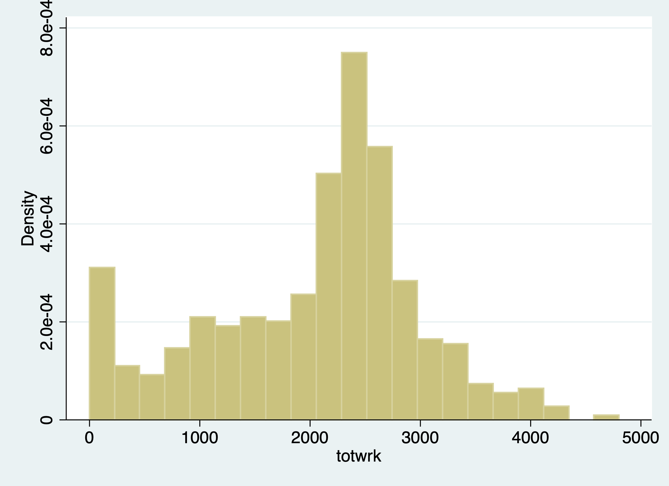
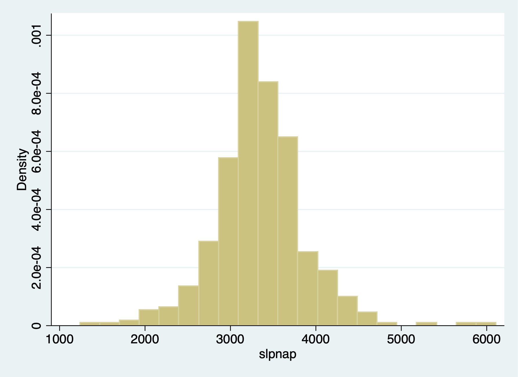
slpnap - total minutes of sleep per week totwrk - total hours of work per year educ - total years of education marr - married dummy variable yngkid - presence of a young child dummy variable gdhlth - “good health” dummy variable
After we set up our panel, we can control for the unobserved cross-sectional unit effect a_i, or unobserved individual effect that do not vary over time. This is all characteristics of the cross-sectional unit of observation that is constant over time or time-invariant.
We are interested in the tradeoff between work and sleep. Our dependent variable of interest is total minutes sleeping per week. Our explanatory variable of interest is the total working hours during the year.
. histogram totwrk
(bin=21, start=0, width=228.80952)

. graph export "/Users/Sam/Desktop/Econ 645/Stata/totwrk.png", replace
(file /Users/Sam/Desktop/Econ 645/Stata/totwrk.png written in PNG format)
. histogram slpnap
(bin=21, start=1240, width=231.90476)

. graph export "/Users/Sam/Desktop/Econ 645/Stata/slpnap.png", replace
(file /Users/Sam/Desktop/Econ 645/Stata/slpnap.png written in PNG format)
When we run OLS, we do not control for unobserved individual time-invariant effects Pooled OLS
. est clear

. eststo OLS: reg slpnap i.d81 totwrk educ marr yngkid gdhlth

      Source │       SS           df       MS      Number of obs   =       478
─────────────┼──────────────────────────────────   F(6, 471)       =      8.50
       Model │  12812772.5         6  2135462.09   Prob > F        =    0.0000
    Residual │   118370944       471  251318.353   R-squared       =    0.0977
─────────────┼──────────────────────────────────   Adj R-squared   =    0.0862
       Total │   131183717       477  275018.274   Root MSE        =    501.32

─────────────┬────────────────────────────────────────────────────────────────
      slpnap │      Coef.   Std. Err.      t    P>|t|     [95% Conf. Interval]
─────────────┼────────────────────────────────────────────────────────────────
       1.d81 │  -77.02965   47.96519    -1.61   0.109    -171.2819    17.22259
      totwrk │  -.1500954   .0244002    -6.15   0.000    -.1980421   -.1021487
        educ │  -20.25655   8.000179    -2.53   0.012    -35.97701   -4.536091
        marr │  -42.19389   53.07869    -0.79   0.427    -146.4942    62.10645
      yngkid │    74.2579   77.32582     0.96   0.337    -77.68838    226.2042
      gdhlth │   29.03733   59.57889     0.49   0.626    -88.03599    146.1107
       _cons │   3958.756   121.7663    32.51   0.000     3719.483    4198.028
─────────────┴────────────────────────────────────────────────────────────────
FD Model
. eststo FD: reg d.slpnap d.totwrk d.educ d.marr d.yngkid d.gdhlth

      Source │       SS           df       MS      Number of obs   =       239
─────────────┼──────────────────────────────────   F(5, 233)       =      8.19
       Model │  14674698.2         5  2934939.64   Prob > F        =    0.0000
    Residual │  83482611.7       233  358294.471   R-squared       =    0.1495
─────────────┼──────────────────────────────────   Adj R-squared   =    0.1313
       Total │  98157309.9       238  412425.672   Root MSE        =    598.58

─────────────┬────────────────────────────────────────────────────────────────
    D.slpnap │      Coef.   Std. Err.      t    P>|t|     [95% Conf. Interval]
─────────────┼────────────────────────────────────────────────────────────────
      totwrk │
         D1. │  -.2266694    .036054    -6.29   0.000    -.2977029   -.1556359
             │
        educ │
         D1. │  -.0244717   48.75938    -0.00   1.000    -96.09008    96.04113
             │
        marr │
         D1. │   104.2139   92.85536     1.12   0.263    -78.72946    287.1574
             │
      yngkid │
         D1. │    94.6654   87.65252     1.08   0.281    -78.02739    267.3582
             │
      gdhlth │
         D1. │   87.57785   76.59913     1.14   0.254    -63.33758    238.4933
             │
       _cons │  -92.63404    45.8659    -2.02   0.045    -182.9989   -2.269152
─────────────┴────────────────────────────────────────────────────────────────
Similar except time dummy and base intercepts look at the difference between educ in Pooled and FE models There is likely a confounder between ability sleep and education
. esttab OLS FD, mtitles se scalars(F r2) drop(0.d81)

────────────────────────────────────────────
                      (1)             (2)
                      OLS              FD
────────────────────────────────────────────
1.d81              -77.03
                  (47.97)

totwrk             -0.150***
                 (0.0244)

educ               -20.26*
                  (8.000)

marr               -42.19
                  (53.08)

yngkid              74.26
                  (77.33)

gdhlth              29.04
                  (59.58)

D.totwrk                           -0.227***
                                 (0.0361)

D.educ                            -0.0245
                                  (48.76)

D.marr                              104.2
                                  (92.86)

D.yngkid                            94.67
                                  (87.65)

D.gdhlth                            87.58
                                  (76.60)

_cons              3958.8***       -92.63*
                  (121.8)         (45.87)
────────────────────────────────────────────
N                     478             239
F                   8.497           8.191
r2                 0.0977           0.150
────────────────────────────────────────────
Standard errors in parentheses
* p<0.05, ** p<0.01, *** p<0.001
Let’s look at elasticities
. gen lnslpnap=ln(slpnap)

. gen lntotwrk=ln(totwrk)
(31 missing values generated)

. gen lneduc=ln(educ)
FD Model
. reg d.lnslpnap d.lntotwrk d.lneduc d.marr d.yngkid d.gdhlth

      Source │       SS           df       MS      Number of obs   =       214
─────────────┼──────────────────────────────────   F(5, 208)       =      4.17
       Model │  .805249181         5  .161049836   Prob > F        =    0.0012
    Residual │  8.03583239       208   .03863381   R-squared       =    0.0911
─────────────┼──────────────────────────────────   Adj R-squared   =    0.0692
       Total │  8.84108157       213  .041507425   Root MSE        =    .19655

─────────────┬────────────────────────────────────────────────────────────────
  D.lnslpnap │      Coef.   Std. Err.      t    P>|t|     [95% Conf. Interval]
─────────────┼────────────────────────────────────────────────────────────────
    lntotwrk │
         D1. │  -.0848256   .0206499    -4.11   0.000    -.1255354   -.0441158
             │
      lneduc │
         D1. │  -.0289507   .2628724    -0.11   0.912    -.5471864     .489285
             │
        marr │
         D1. │  -.0038529   .0323002    -0.12   0.905    -.0675306    .0598247
             │
      yngkid │
         D1. │   .0056761   .0290466     0.20   0.845    -.0515874    .0629397
             │
      gdhlth │
         D1. │    .048008   .0266772     1.80   0.073    -.0045843    .1006004
             │
       _cons │  -.0204204   .0155593    -1.31   0.191    -.0510947    .0102538
─────────────┴────────────────────────────────────────────────────────────────
A 1% increase in total hours worked leads to a (1.01^-0.0848256)-1)*100=-0.08% decrease in minutes of sleep per week
We will get into time series later in the course, but we will have a preview. With panel data, we are able to see the same observation over time. Given this We can see if lagged values affect current values for the cross-sectional unit of observation.
Eide(1994) wants to assess if prior clear-up rates for crime have a relationship with crime rates in the current time period. The dependent variable of interest is the current period crime rate. The variable of interest is the clear-up percentage which is the rate of crimes that have lead to conviction.
. use crime3.dta, clear
We will use a log-log model and use a first-difference
. reg clcrime cclrprc1 cclrprc2

      Source │       SS           df       MS      Number of obs   =        53
─────────────┼──────────────────────────────────   F(2, 50)        =      5.99
       Model │  1.42294697         2  .711473484   Prob > F        =    0.0046
    Residual │  5.93723904        50  .118744781   R-squared       =    0.1933
─────────────┼──────────────────────────────────   Adj R-squared   =    0.1611
       Total │  7.36018601        52  .141542039   Root MSE        =    .34459

─────────────┬────────────────────────────────────────────────────────────────
     clcrime │      Coef.   Std. Err.      t    P>|t|     [95% Conf. Interval]
─────────────┼────────────────────────────────────────────────────────────────
    cclrprc1 │  -.0040475   .0047199    -0.86   0.395    -.0135276    .0054326
    cclrprc2 │  -.0131966   .0051946    -2.54   0.014    -.0236302   -.0027629
       _cons │   .0856556   .0637825     1.34   0.185    -.0424553    .2137665
─────────────┴────────────────────────────────────────────────────────────────
Our model tells us that 1 percent increase in getting crimes to conviction leads to a reduction in the current period crime rate of about ((1.01^-0.013196)-1)*100%=-0.0132 percent. Assuming this model is specified well, crime rates are sensitive to clear-up rates from the prior 2 years.
We should test for heteroskedasticity and serial correlation when running our First-Difference Estimator.
Serial correlation means that the differences in the idiosyncractic errors between time periods are correlated, which is a violation of our assumption that there is no serial correlation for our first-difference estimator
We’ll use data from Papke (1994) who studied the effect of Indiana’s enterprise zone program on unemployment claims. Do enterprise zones increase employment and reduce unemployment claims?
She analyzes 22 cities in Indiana from 1980 to 1988, since 6 enterprise zones were established in 1984. Twelve cities did not receive the enterprise zones, while 10 cities did get enterprise zones.
. use "ezunem.dta", clear
We’ll use a simple analysis that the change in natural log of unemployment claims is a function of time period binaries, change in enterprise zones, and the idiosyncractic error.
One way to do it is to use the data already created. Pooled OLS
. reg luclms i.d82 i.d83 i.d84 i.d85 i.d86 i.d87 i.d88 cez

      Source │       SS           df       MS      Number of obs   =       176
─────────────┼──────────────────────────────────   F(8, 167)       =     10.39
       Model │  29.2551235         8  3.65689043   Prob > F        =    0.0000
    Residual │  58.7753327       167    .3519481   R-squared       =    0.3323
─────────────┼──────────────────────────────────   Adj R-squared   =    0.3003
       Total │  88.0304561       175  .503031178   Root MSE        =    .59325

─────────────┬────────────────────────────────────────────────────────────────
      luclms │      Coef.   Std. Err.      t    P>|t|     [95% Conf. Interval]
─────────────┼────────────────────────────────────────────────────────────────
       1.d82 │   .4571276   .1788722     2.56   0.011     .1039853    .8102699
       1.d83 │   .1023765   .1788722     0.57   0.568    -.2507658    .4555188
       1.d84 │  -.2821805   .1882109    -1.50   0.136    -.6537598    .0893988
       1.d85 │  -.3150721   .1830816    -1.72   0.087    -.6765248    .0463805
       1.d86 │  -.3470941   .1788722    -1.94   0.054    -.7002364    .0060481
       1.d87 │   -.614778   .1788722    -3.44   0.001    -.9679202   -.2616357
       1.d88 │  -.9534624   .1788722    -5.33   0.000    -1.306605   -.6003201
         cez │  -.0139924   .2146822    -0.07   0.948    -.4378332    .4098484
       _cons │   11.37276   .1264818    89.92   0.000     11.12305    11.62247
─────────────┴────────────────────────────────────────────────────────────────
Let’s say we didn’t have the data already created. What we’ll need to do is to set the panel data with xtset unit timeperiod Set the Panel Data
. xtset city year
       panel variable:  city (strongly balanced)
        time variable:  year, 1980 to 1988
                delta:  1 unit
We can use the d. operator to use a first difference First Difference
. reg d.luclms i.d82 i.d83 i.d84 i.d85 i.d86 i.d87 i.d88 d.ez

      Source │       SS           df       MS      Number of obs   =       176
─────────────┼──────────────────────────────────   F(8, 167)       =     34.50
       Model │  12.8826331         8  1.61032914   Prob > F        =    0.0000
    Residual │  7.79583815       167  .046681666   R-squared       =    0.6230
─────────────┼──────────────────────────────────   Adj R-squared   =    0.6049
       Total │  20.6784713       175  .118162693   Root MSE        =    .21606

─────────────┬────────────────────────────────────────────────────────────────
    D.luclms │      Coef.   Std. Err.      t    P>|t|     [95% Conf. Interval]
─────────────┼────────────────────────────────────────────────────────────────
       1.d82 │   .7787595   .0651444    11.95   0.000     .6501469    .9073721
       1.d83 │  -.0331192   .0651444    -0.51   0.612    -.1617318    .0954934
       1.d84 │  -.0171382   .0685455    -0.25   0.803    -.1524655    .1181891
       1.d85 │    .323081   .0666774     4.85   0.000     .1914417    .4547202
       1.d86 │    .292154   .0651444     4.48   0.000     .1635413    .4207666
       1.d87 │   .0539481   .0651444     0.83   0.409    -.0746645    .1825607
       1.d88 │  -.0170526   .0651444    -0.26   0.794    -.1456652    .1115601
             │
          ez │
         D1. │  -.1818775   .0781862    -2.33   0.021    -.3362382   -.0275169
             │
       _cons │  -.3216319    .046064    -6.98   0.000    -.4125748   -.2306891
─────────────┴────────────────────────────────────────────────────────────────
Test for Heteroskedasticity Bruesch-Pagan/Cameron-Trivedi Test
. estat imtest

Cameron & Trivedi's decomposition of IM-test

─────────────────────┬─────────────────────────────
              Source │       chi2     df      p
─────────────────────┼─────────────────────────────
  Heteroskedasticity │      12.85      9    0.1697
            Skewness │      13.04      8    0.1104
            Kurtosis │       0.11      1    0.7414
─────────────────────┼─────────────────────────────
               Total │      26.00     18    0.0998
─────────────────────┴─────────────────────────────
White Test
. estat imtest, white

White's test for Ho: homoskedasticity
         against Ha: unrestricted heteroskedasticity

         chi2(9)      =     12.85
         Prob > chi2  =    0.1697

Cameron & Trivedi's decomposition of IM-test

─────────────────────┬─────────────────────────────
              Source │       chi2     df      p
─────────────────────┼─────────────────────────────
  Heteroskedasticity │      12.85      9    0.1697
            Skewness │      13.04      8    0.1104
            Kurtosis │       0.11      1    0.7414
─────────────────────┼─────────────────────────────
               Total │      26.00     18    0.0998
─────────────────────┴─────────────────────────────
We fail to reject the null hypothesis of homoskedastic standard errors.
Test for autocorrelation We can use the command xtserial to test for serial correlation, since we already set up our panel above.
. help xtserial

. xtserial luclms d83 d84 d85 d86 d87 d88 cez, output

Linear regression                               Number of obs     =        154
                                                F(7, 21)          =     102.85
                                                Prob > F          =     0.0000
                                                R-squared         =     0.4711
                                                Root MSE          =     .28063

                                  (Std. Err. adjusted for 22 clusters in city)
─────────────┬────────────────────────────────────────────────────────────────
             │               Robust
    D.luclms │      Coef.   Std. Err.      t    P>|t|     [95% Conf. Interval]
─────────────┼────────────────────────────────────────────────────────────────
         d83 │
         D1. │  -.3547511   .0410541    -8.64   0.000    -.4401277   -.2693745
             │
         d84 │
         D1. │  -.7240107   .0816269    -8.87   0.000     -.893763   -.5542583
             │
         d85 │
         D1. │  -.7620015   .0540757   -14.09   0.000    -.8744581   -.6495448
             │
         d86 │
         D1. │  -.8042218   .0490039   -16.41   0.000     -.906131   -.7023126
             │
         d87 │
         D1. │  -1.071906   .0496977   -21.57   0.000    -1.175258   -.9685535
             │
         d88 │
         D1. │   -1.41059    .065833   -21.43   0.000    -1.547497   -1.273683
             │
         cez │
         D1. │   -.070083   .0650804    -1.08   0.294     -.205425     .065259
─────────────┴────────────────────────────────────────────────────────────────

Wooldridge test for autocorrelation in panel data
H0: no first-order autocorrelation
    F(  1,      21) =    120.981
           Prob > F =      0.0000
We reject the null hypothesis that the differences in idiosyncratic errors is 0.
What can we do for this serial correlation? We can cluster our standard errors to account for the serial correlation within units.
Robust for serial correlation within unit of analysis clusters
. reg d.luclms i.d82 i.d83 i.d84 i.d85 i.d86 i.d87 i.d88 d.cez, robust cluster(city)
note: 1.d88 omitted because of collinearity

Linear regression                               Number of obs     =        154
                                                F(7, 21)          =      41.20
                                                Prob > F          =     0.0000
                                                R-squared         =     0.6333
                                                Root MSE          =     .21865

                                  (Std. Err. adjusted for 22 clusters in city)
─────────────┬────────────────────────────────────────────────────────────────
             │               Robust
    D.luclms │      Coef.   Std. Err.      t    P>|t|     [95% Conf. Interval]
─────────────┼────────────────────────────────────────────────────────────────
       1.d82 │   .7958121   .0577076    13.79   0.000     .6758025    .9158217
       1.d83 │  -.0160666   .0565946    -0.28   0.779    -.1337615    .1016282
       1.d84 │  -.0305751   .0742049    -0.41   0.684    -.1848926    .1237424
       1.d85 │   .3006937   .0568959     5.28   0.000     .1823723    .4190151
       1.d86 │   .2964642   .0786548     3.77   0.001     .1328926    .4600357
       1.d87 │   .0710007   .0462206     1.54   0.139    -.0251204    .1671217
       1.d88 │          0  (omitted)
             │
         cez │
         D1. │   -.070083   .0653029    -1.07   0.295    -.2058877    .0657217
             │
       _cons │  -.3386845   .0359416    -9.42   0.000    -.4134292   -.2639397
─────────────┴────────────────────────────────────────────────────────────────
Once we account for the serial correlation in the idiosyncratic error, our coefficient on the change in enterprise zone becomes statistically insignificant.
Testing for serial correlation, and Clustering your standard error at the treatment level is an important test and step with FD estimators.
When we get to Fixed Effects (Within) estimator, the assumption is slightly different. For First-Difference Estimator, the DIFFERENCE in idiosyncratic errors cannot be correlated, but for Fixed-Effects (Within) Estimator the assumption states that only the idiosyncratic errors cannot be correlated.
Cornwell and Trumbull (1994) analyzed data on 90 counties in North Carolina from 1981 to 1987 to using panel data to account for time-invariant effects. Their cross-sectional unit of observation is the county (not individuals within a county). They want to know what the is the effect of police per capita on crime rates.
For our model the dependent variable is the change in the natural log of crimes per person (lcrimrte). They are interested in estimating the sensitivity of police per capita (polpc) on crime rate, so they use the difference in natural log of police per capita. This will get you elasticities, which provide useful interpretations of percentage increases.
They also control for the difference in natural log of probability of arrest (prbarr), the probability of conviction (prbconv), the probability of serving time in prison given a conviction (prbpris), and the average sentence length.
. use "crime4.dta", clear
Pooled OLS
. reg lcrmrte i.d82 i.d83 i.d84 i.d85 i.d86 i.d87 lprbarr lprbconv lprbpris lavgsen lpolpc

      Source │       SS           df       MS      Number of obs   =       630
─────────────┼──────────────────────────────────   F(11, 618)      =     74.49
       Model │  117.644669        11  10.6949699   Prob > F        =    0.0000
    Residual │   88.735673       618  .143585231   R-squared       =    0.5700
─────────────┼──────────────────────────────────   Adj R-squared   =    0.5624
       Total │  206.380342       629  .328108652   Root MSE        =    .37893

─────────────┬────────────────────────────────────────────────────────────────
     lcrmrte │      Coef.   Std. Err.      t    P>|t|     [95% Conf. Interval]
─────────────┼────────────────────────────────────────────────────────────────
       1.d82 │   .0051371    .057931     0.09   0.929    -.1086284    .1189026
       1.d83 │   -.043503   .0576243    -0.75   0.451    -.1566662    .0696601
       1.d84 │  -.1087542    .057923    -1.88   0.061     -.222504    .0049957
       1.d85 │  -.0780454   .0583244    -1.34   0.181    -.1925835    .0364928
       1.d86 │  -.0420791   .0578218    -0.73   0.467      -.15563    .0714719
       1.d87 │  -.0270426    .056899    -0.48   0.635    -.1387815    .0846963
     lprbarr │  -.7195033   .0367657   -19.57   0.000    -.7917042   -.6473024
    lprbconv │  -.5456589   .0263683   -20.69   0.000    -.5974413   -.4938765
    lprbpris │   .2475521   .0672268     3.68   0.000     .1155314    .3795728
     lavgsen │  -.0867575   .0579205    -1.50   0.135    -.2005023    .0269872
      lpolpc │   .3659886   .0300252    12.19   0.000     .3070248    .4249525
       _cons │  -2.082293   .2516253    -8.28   0.000    -2.576438   -1.588149
─────────────┴────────────────────────────────────────────────────────────────
First Difference
. xtset county year
       panel variable:  county (strongly balanced)
        time variable:  year, 81 to 87
                delta:  1 unit
With xtset, we can use the d. for our explanatory variables First-Difference
. reg d.lcrmrte i.d83 i.d84 i.d85 i.d86 i.d87 d.lprbarr d.lprbconv d.lprbpris d.lavgsen d.lpolpc

      Source │       SS           df       MS      Number of obs   =       540
─────────────┼──────────────────────────────────   F(10, 529)      =     40.32
       Model │  9.60042828        10  .960042828   Prob > F        =    0.0000
    Residual │  12.5963755       529  .023811674   R-squared       =    0.4325
─────────────┼──────────────────────────────────   Adj R-squared   =    0.4218
       Total │  22.1968038       539  .041181454   Root MSE        =    .15431

─────────────┬────────────────────────────────────────────────────────────────
   D.lcrmrte │      Coef.   Std. Err.      t    P>|t|     [95% Conf. Interval]
─────────────┼────────────────────────────────────────────────────────────────
       1.d83 │  -.0998658   .0238953    -4.18   0.000    -.1468071   -.0529246
       1.d84 │  -.0479374   .0235021    -2.04   0.042    -.0941063   -.0017686
       1.d85 │  -.0046111   .0234998    -0.20   0.845    -.0507756    .0415533
       1.d86 │   .0275143   .0241494     1.14   0.255    -.0199261    .0749548
       1.d87 │   .0408267   .0244153     1.67   0.095    -.0071361    .0887895
             │
     lprbarr │
         D1. │  -.3274942   .0299801   -10.92   0.000    -.3863889   -.2685994
             │
    lprbconv │
         D1. │  -.2381066   .0182341   -13.06   0.000    -.2739268   -.2022864
             │
    lprbpris │
         D1. │  -.1650462    .025969    -6.36   0.000    -.2160613   -.1140312
             │
     lavgsen │
         D1. │  -.0217607   .0220909    -0.99   0.325    -.0651574     .021636
             │
      lpolpc │
         D1. │   .3984264    .026882    14.82   0.000     .3456177     .451235
             │
       _cons │   .0077134   .0170579     0.45   0.651    -.0257961    .0412229
─────────────┴────────────────────────────────────────────────────────────────
So our model is estimating that a 1% increase in police per capita increases the crime rate by about 0.4%. We would expect that increases in police per capita would reduce crime rates. This is likely shows that there are problems in our model.
What is happening? Likely simultaneity bias is occurring. Areas with high crime rates have more police per capita, which more police per capita is associated with higher crime rates. It’s a circular/endogenous reference, so we will need an valid instrument to deal with this simultaneity bias/endogeneity.
We can test for heteroskedasticity and serial correlation, but this only affects our standard errors, not our coefficients.
Test for autocorrelation with one lag AR(1) We can see that serial correlation is a problem, which means we should cluster our standard errors at the county level.
. predict r, residual
(90 missing values generated)

. gen lag_r =l.r
(180 missing values generated)

. reg r lag_r i.d83 i.d84 i.d85 i.d86 i.d87 d.lprbarr d.lprbconv d.lprbpris d.lavgsen d.lpolpc
note: 1.d87 omitted because of collinearity

      Source │       SS           df       MS      Number of obs   =       450
─────────────┼──────────────────────────────────   F(10, 439)      =      2.35
       Model │  .564663971        10  .056466397   Prob > F        =    0.0102
    Residual │   10.528838       439  .023983686   R-squared       =    0.0509
─────────────┼──────────────────────────────────   Adj R-squared   =    0.0293
       Total │   11.093502       449  .024707131   Root MSE        =    .15487

─────────────┬────────────────────────────────────────────────────────────────
           r │      Coef.   Std. Err.      t    P>|t|     [95% Conf. Interval]
─────────────┼────────────────────────────────────────────────────────────────
       lag_r │  -.2332117   .0488802    -4.77   0.000      -.32928   -.1371435
       1.d83 │  -.0012379   .0234019    -0.05   0.958    -.0472317    .0447558
       1.d84 │  -.0016543   .0236303    -0.07   0.944    -.0480968    .0447883
       1.d85 │  -.0006044   .0236114    -0.03   0.980    -.0470098    .0458009
       1.d86 │   .0008841   .0233216     0.04   0.970    -.0449517    .0467199
       1.d87 │          0  (omitted)
             │
     lprbarr │
         D1. │   .0082875   .0330698     0.25   0.802    -.0567074    .0732823
             │
    lprbconv │
         D1. │  -.0036161   .0200155    -0.18   0.857    -.0429542    .0357221
             │
    lprbpris │
         D1. │   .0017131    .027855     0.06   0.951    -.0530326    .0564588
             │
     lavgsen │
         D1. │  -.0125831   .0245006    -0.51   0.608    -.0607362      .03557
             │
      lpolpc │
         D1. │   .0214883   .0282688     0.76   0.448    -.0340706    .0770473
             │
       _cons │   .0005347   .0167411     0.03   0.975     -.032368    .0334373
─────────────┴────────────────────────────────────────────────────────────────
We can always use our xtserial command to test for AR(1) serial correlation.
. reg d.lcrmrte i.d83 i.d84 i.d85 i.d86 i.d87 d.lprbarr d.lprbconv d.lprbpris d.lavgsen d.lpolpc

      Source │       SS           df       MS      Number of obs   =       540
─────────────┼──────────────────────────────────   F(10, 529)      =     40.32
       Model │  9.60042828        10  .960042828   Prob > F        =    0.0000
    Residual │  12.5963755       529  .023811674   R-squared       =    0.4325
─────────────┼──────────────────────────────────   Adj R-squared   =    0.4218
       Total │  22.1968038       539  .041181454   Root MSE        =    .15431

─────────────┬────────────────────────────────────────────────────────────────
   D.lcrmrte │      Coef.   Std. Err.      t    P>|t|     [95% Conf. Interval]
─────────────┼────────────────────────────────────────────────────────────────
       1.d83 │  -.0998658   .0238953    -4.18   0.000    -.1468071   -.0529246
       1.d84 │  -.0479374   .0235021    -2.04   0.042    -.0941063   -.0017686
       1.d85 │  -.0046111   .0234998    -0.20   0.845    -.0507756    .0415533
       1.d86 │   .0275143   .0241494     1.14   0.255    -.0199261    .0749548
       1.d87 │   .0408267   .0244153     1.67   0.095    -.0071361    .0887895
             │
     lprbarr │
         D1. │  -.3274942   .0299801   -10.92   0.000    -.3863889   -.2685994
             │
    lprbconv │
         D1. │  -.2381066   .0182341   -13.06   0.000    -.2739268   -.2022864
             │
    lprbpris │
         D1. │  -.1650462    .025969    -6.36   0.000    -.2160613   -.1140312
             │
     lavgsen │
         D1. │  -.0217607   .0220909    -0.99   0.325    -.0651574     .021636
             │
      lpolpc │
         D1. │   .3984264    .026882    14.82   0.000     .3456177     .451235
             │
       _cons │   .0077134   .0170579     0.45   0.651    -.0257961    .0412229
─────────────┴────────────────────────────────────────────────────────────────
. xtserial lcrmrte d83 d84 d85 d86 d87 lprbarr lprbconv lprbpris lavgsen lpolpc, output

Linear regression                               Number of obs     =        540
                                                F(10, 89)         =      13.68
                                                Prob > F          =     0.0000
                                                R-squared         =     0.4323
                                                Root MSE          =     .15419

                                (Std. Err. adjusted for 90 clusters in county)
─────────────┬────────────────────────────────────────────────────────────────
             │               Robust
   D.lcrmrte │      Coef.   Std. Err.      t    P>|t|     [95% Conf. Interval]
─────────────┼────────────────────────────────────────────────────────────────
         d83 │
         D1. │  -.0920147   .0146354    -6.29   0.000     -.121095   -.0629345
             │
         d84 │
         D1. │  -.1323557   .0179759    -7.36   0.000    -.1680734    -.096638
             │
         d85 │
         D1. │  -.1293278   .0232716    -5.56   0.000    -.1755679   -.0830876
             │
         d86 │
         D1. │  -.0938692   .0209561    -4.48   0.000    -.1355086   -.0522298
             │
         d87 │
         D1. │  -.0449434   .0236533    -1.90   0.061     -.091942    .0020552
             │
     lprbarr │
         D1. │  -.3263268   .0561808    -5.81   0.000     -.437957   -.2146967
             │
    lprbconv │
         D1. │  -.2375214   .0392585    -6.05   0.000    -.3155272   -.1595155
             │
    lprbpris │
         D1. │  -.1645109   .0457092    -3.60   0.001     -.255334   -.0736878
             │
     lavgsen │
         D1. │  -.0246909   .0252756    -0.98   0.331    -.0749129    .0255312
             │
      lpolpc │
         D1. │   .3976861   .1024878     3.88   0.000     .1940451    .6013271
─────────────┴────────────────────────────────────────────────────────────────

Wooldridge test for autocorrelation in panel data
H0: no first-order autocorrelation
    F(  1,      89) =     22.065
           Prob > F =      0.0000
We can also test for heteroskedasticity
. reg d.lcrmrte i.d83 i.d84 i.d85 i.d86 i.d87 d.lprbarr d.lprbconv d.lprbpris d.lavgsen d.lpolpc
Source │ SS df MS Number of obs = 540
─────────────┼────────────────────────────────── F(10, 529) = 40.32
Model │ 9.60042828 10 .960042828 Prob > F = 0.0000
Residual │ 12.5963755 529 .023811674 R-squared = 0.4325
─────────────┼────────────────────────────────── Adj R-squared = 0.4218
Total │ 22.1968038 539 .041181454 Root MSE = .15431
─────────────┬────────────────────────────────────────────────────────────────
D.lcrmrte │ Coef. Std. Err. t P>|t| [95% Conf. Interval]
─────────────┼────────────────────────────────────────────────────────────────
1.d83 │ -.0998658 .0238953 -4.18 0.000 -.1468071 -.0529246
1.d84 │ -.0479374 .0235021 -2.04 0.042 -.0941063 -.0017686
1.d85 │ -.0046111 .0234998 -0.20 0.845 -.0507756 .0415533
1.d86 │ .0275143 .0241494 1.14 0.255 -.0199261 .0749548
1.d87 │ .0408267 .0244153 1.67 0.095 -.0071361 .0887895
│
lprbarr │
D1. │ -.3274942 .0299801 -10.92 0.000 -.3863889 -.2685994
│
lprbconv │
D1. │ -.2381066 .0182341 -13.06 0.000 -.2739268 -.2022864
│
lprbpris │
D1. │ -.1650462 .025969 -6.36 0.000 -.2160613 -.1140312
│
lavgsen │
D1. │ -.0217607 .0220909 -0.99 0.325 -.0651574 .021636
│
lpolpc │
D1. │ .3984264 .026882 14.82 0.000 .3456177 .451235
│
_cons │ .0077134 .0170579 0.45 0.651 -.0257961 .0412229
─────────────┴────────────────────────────────────────────────────────────────
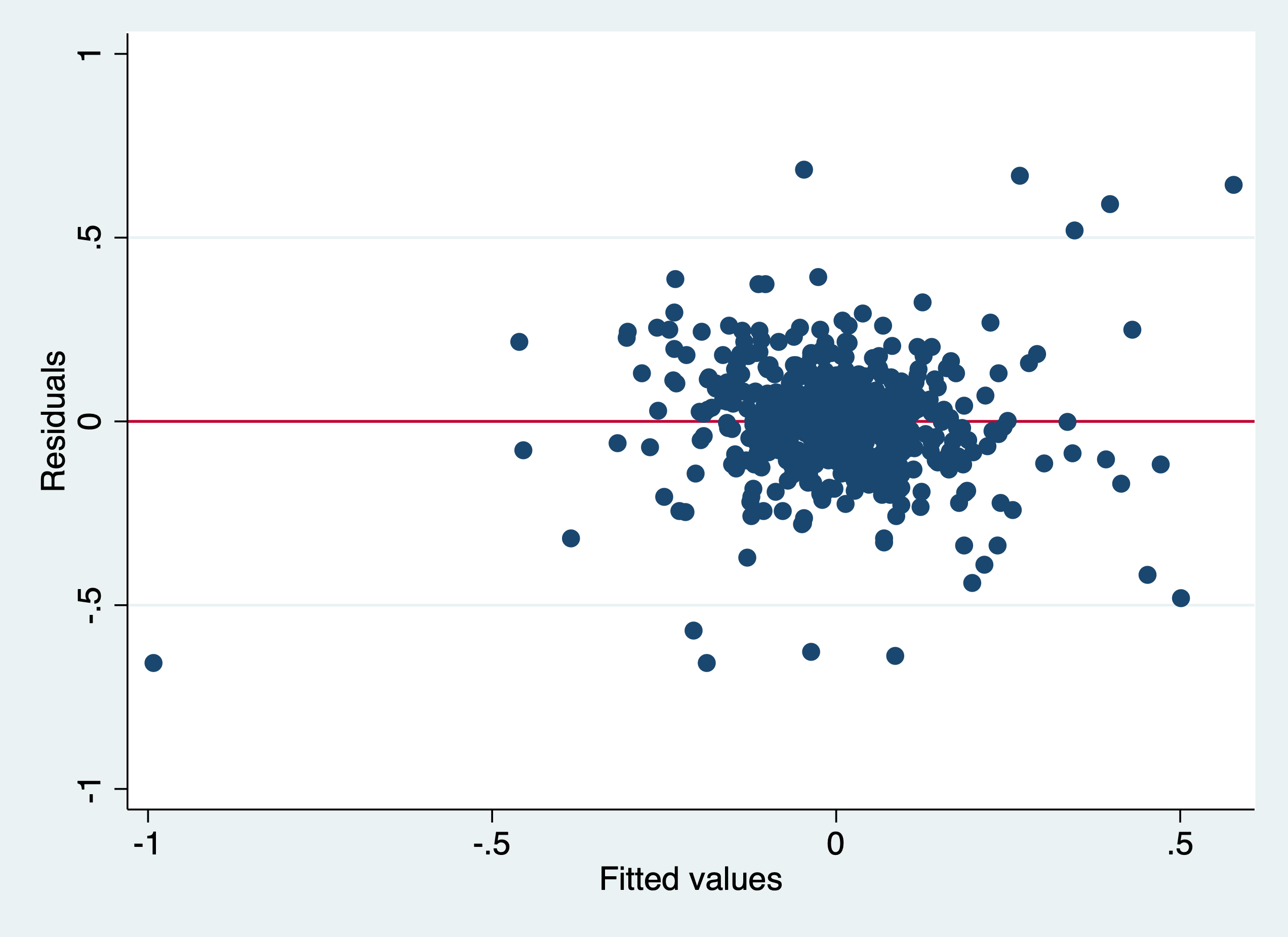
. rvfplot,yline(0)
. graph export "/Users/Sam/Desktop/Econ 645/Stata/week3_htsk.png", replace
(file /Users/Sam/Desktop/Econ 645/Stata/week3_htsk.png written in PNG format)
 We can use the
White Test and Breusch-Pagan, which yield different results
We can use the
White Test and Breusch-Pagan, which yield different results
. estat imtest, white

White's test for Ho: homoskedasticity
         against Ha: unrestricted heteroskedasticity

         chi2(50)     =    257.57
         Prob > chi2  =    0.0000

Cameron & Trivedi's decomposition of IM-test

─────────────────────┬─────────────────────────────
              Source │       chi2     df      p
─────────────────────┼─────────────────────────────
  Heteroskedasticity │     257.57     50    0.0000
            Skewness │      62.96     10    0.0000
            Kurtosis │      12.82      1    0.0003
─────────────────────┼─────────────────────────────
               Total │     333.35     61    0.0000
─────────────────────┴─────────────────────────────

. estat hettest

Breusch-Pagan / Cook-Weisberg test for heteroskedasticity
         Ho: Constant variance
         Variables: fitted values of D.lcrmrte

         chi2(1)      =     1.16
         Prob > chi2  =   0.2807
Re-estimate with Robust Standard Errors clustered at the county level and cluster by county (deal with error correlations within counties)
. reg d.lcrmrte i.d83 i.d84 i.d85 i.d86 i.d87 d.lprbarr d.lprbconv d.lprbpris d.lavgsen d.lpolpc, robust cluster(
> county)

Linear regression                               Number of obs     =        540
                                                F(10, 89)         =      13.56
                                                Prob > F          =     0.0000
                                                R-squared         =     0.4325
                                                Root MSE          =     .15431

                                (Std. Err. adjusted for 90 clusters in county)
─────────────┬────────────────────────────────────────────────────────────────
             │               Robust
   D.lcrmrte │      Coef.   Std. Err.      t    P>|t|     [95% Conf. Interval]
─────────────┼────────────────────────────────────────────────────────────────
       1.d83 │  -.0998658   .0222563    -4.49   0.000    -.1440887    -.055643
       1.d84 │  -.0479374   .0200531    -2.39   0.019    -.0877825   -.0080923
       1.d85 │  -.0046111     .02503    -0.18   0.854    -.0543453     .045123
       1.d86 │   .0275143   .0211829     1.30   0.197    -.0145756    .0696043
       1.d87 │   .0408267   .0241102     1.69   0.094    -.0070797    .0887331
             │
     lprbarr │
         D1. │  -.3274942   .0564281    -5.80   0.000    -.4396157   -.2153727
             │
    lprbconv │
         D1. │  -.2381066   .0395843    -6.02   0.000    -.3167598   -.1594534
             │
    lprbpris │
         D1. │  -.1650462   .0457923    -3.60   0.001    -.2560345    -.074058
             │
     lavgsen │
         D1. │  -.0217607     .02582    -0.84   0.402    -.0730644     .029543
             │
      lpolpc │
         D1. │   .3984264   .1029342     3.87   0.000     .1938983    .6029545
             │
       _cons │   .0077134   .0137846     0.56   0.577    -.0196763     .035103
─────────────┴────────────────────────────────────────────────────────────────
Even accounting for heteroskedasticity and serial correlation, our model is likely biased by simultaneity bias.
Honestly, this chapter has a bunch of useful information, but the most important parts are label define and its two options of add and modify, along with label values. Everything else is interesting, but not essential. Section 5.8 on formatting is also fairly important for down the road.
. cd "/Users/Sam/Desktop/Econ 645/Data/Mitchell"
/Users/Sam/Desktop/Econ 645/Data/Mitchell
Let’s get some data on the survey of graduate students
. use "survey7.dta", clear
(Survey of graduate students)
We have seen the describe command before, but it is a very useful command to being working with data. It provides the varible name, storage type, display format, value label, and variable lable
. describe

Contains data from survey7.dta
  obs:             8                          Survey of graduate students
 vars:            11                          5 May 2020 14:37
 size:           400                          (_dta has notes)
─────────────────────────────────────────────────────────────────────────────────────────────────────────────────
              storage   display    value
variable name   type    format     label      variable label
─────────────────────────────────────────────────────────────────────────────────────────────────────────────────
id              float   %9.0g                 Unique identification variable
STUDENTVARS     float   %9.0g                 STUDENT VARIABLES ===============
gender          float   %9.0g      mf         Gender of student
race            float   %19.0g     racelab  * Race of student
bday            float   %td..                 Date of birth of student
income          float   %11.1fc               Income of student
havechild       float   %18.0g     havelab  * Given birth to a child?
KIDVARS         float   %9.0g                 KID VARIABLES ===================
kidname         str10   %-10s                 Name of child
ksex            float   %15.0g     mfkid    * Sex of child
kbday           float   %td..                 Date of birth of child
                                            * indicated variables have notes
─────────────────────────────────────────────────────────────────────────────────────────────────────────────────
Sorted by:
We also have a short option, but it just contain general information
. describe, short

Contains data from survey7.dta
  obs:             8                          Survey of graduate students
 vars:            11                          5 May 2020 14:37
 size:           400
Sorted by:
We can subset the variables we want to describe if we want
. describe id gender race

              storage   display    value
variable name   type    format     label      variable label
─────────────────────────────────────────────────────────────────────────────────────────────────────────────────
id              float   %9.0g                 Unique identification variable
gender          float   %9.0g      mf         Gender of student
race            float   %19.0g     racelab  * Race of student
Finally, the command codebook provides a deep dive into your dataset. This is very useful for looking at the value labels. We only see the value label name in the describe command, but the codebook command provides more information, such as type of variable, label name, range of values, unique values, missing, value labels, missing value labels (if any)
. codebook

─────────────────────────────────────────────────────────────────────────────────────────────────────────────────
id                                                                                 Unique identification variable
─────────────────────────────────────────────────────────────────────────────────────────────────────────────────

                  type:  numeric (float)

                 range:  [1,8]                        units:  1
         unique values:  8                        missing .:  0/8

            tabulation:  Freq.  Value
                             1  1
                             1  2
                             1  3
                             1  4
                             1  5
                             1  6
                             1  7
                             1  8

─────────────────────────────────────────────────────────────────────────────────────────────────────────────────
STUDENTVARS                                                                     STUDENT VARIABLES ===============
─────────────────────────────────────────────────────────────────────────────────────────────────────────────────

                  type:  numeric (float)

                 range:  [.,.]                        units:  .
         unique values:  0                        missing .:  8/8

            tabulation:  Freq.  Value
                             8  .

─────────────────────────────────────────────────────────────────────────────────────────────────────────────────
gender                                                                                          Gender of student
─────────────────────────────────────────────────────────────────────────────────────────────────────────────────

                  type:  numeric (float)
                 label:  mf

                 range:  [1,2]                        units:  1
         unique values:  2                        missing .:  0/8

            tabulation:  Freq.   Numeric  Label
                             3         1  Male
                             5         2  Female

─────────────────────────────────────────────────────────────────────────────────────────────────────────────────
race                                                                                              Race of student
─────────────────────────────────────────────────────────────────────────────────────────────────────────────────

                  type:  numeric (float)
                 label:  racelab

                 range:  [1,5]                        units:  1
         unique values:  5                        missing .:  0/8

            tabulation:  Freq.   Numeric  Label
                             2         1  White
                             2         2  Asian
                             2         3  Hispanic
                             1         4  African American
                             1         5  Other

─────────────────────────────────────────────────────────────────────────────────────────────────────────────────
bday                                                                                     Date of birth of student
─────────────────────────────────────────────────────────────────────────────────────────────────────────────────

                  type:  numeric daily date (float)

                 range:  [389,7935]                   units:  1
       or equivalently:  [24jan1961,22sep1981]        units:  days
         unique values:  8                        missing .:  0/8

            tabulation:  Freq.  Value
                             1  389    24jan1961
                             1  3027   15apr1968
                             1  4160   23may1971
                             1  4924   25jun1973
                             1  5036   15oct1973
                             1  6059   03aug1976
                             1  6391   01jul1977
                             1  7935   22sep1981

─────────────────────────────────────────────────────────────────────────────────────────────────────────────────
income                                                                                          Income of student
─────────────────────────────────────────────────────────────────────────────────────────────────────────────────

                  type:  numeric (float)

                 range:  [545.23,1284354.5]           units:  .01
         unique values:  8                        missing .:  0/8

            tabulation:  Freq.  Value
                             1  545.22998
                             1  4500.9199
                             1  10500.93
                             1  45234.129
                             1  109452.11
                             1  120102.32
                             1  124313.45
                             1  1284354.5

─────────────────────────────────────────────────────────────────────────────────────────────────────────────────
havechild                                                                                 Given birth to a child?
─────────────────────────────────────────────────────────────────────────────────────────────────────────────────

                  type:  numeric (float)
                 label:  havelab

                 range:  [0,1]                        units:  1
         unique values:  2                        missing .:  0/8
       unique mv codes:  1                       missing .*:  3/8

            tabulation:  Freq.   Numeric  Label
                             1         0  Dont Have Child
                             4         1  Have Child
                             3        .n  NA

─────────────────────────────────────────────────────────────────────────────────────────────────────────────────
KIDVARS                                                                         KID VARIABLES ===================
─────────────────────────────────────────────────────────────────────────────────────────────────────────────────

                  type:  numeric (float)

                 range:  [.,.]                        units:  .
         unique values:  0                        missing .:  8/8

            tabulation:  Freq.  Value
                             8  .

─────────────────────────────────────────────────────────────────────────────────────────────────────────────────
kidname                                                                                             Name of child
─────────────────────────────────────────────────────────────────────────────────────────────────────────────────

                  type:  string (str10), but longest is str9

         unique values:  5                        missing "":  0/8

            tabulation:  Freq.  Value
                             4  ""
                             1  "Catherine"
                             1  "Robin"
                             1  "Sally"
                             1  "Samuell"

               warning:  variable has leading and trailing blanks

─────────────────────────────────────────────────────────────────────────────────────────────────────────────────
ksex                                                                                                 Sex of child
─────────────────────────────────────────────────────────────────────────────────────────────────────────────────

                  type:  numeric (float)
                 label:  mfkid

                 range:  [1,2]                        units:  1
         unique values:  2                        missing .:  0/8
       unique mv codes:  2                       missing .*:  5/8

            tabulation:  Freq.   Numeric  Label
                             1         1  Male
                             2         2  Female
                             4        .n  NA
                             1        .u  Unknown

─────────────────────────────────────────────────────────────────────────────────────────────────────────────────
kbday                                                                                      Date of birth of child
─────────────────────────────────────────────────────────────────────────────────────────────────────────────────

                  type:  numeric daily date (float)

                 range:  [12888,15932]                units:  1
       or equivalently:  [15apr1995,15aug2003]        units:  days
         unique values:  4                        missing .:  4/8

            tabulation:  Freq.  Value
                             1  12888  15apr1995
                             1  14019  20may1998
                             1  14256  12jan1999
                             1  15932  15aug2003
                             4  .              .
We can go by variables
. codebook race

─────────────────────────────────────────────────────────────────────────────────────────────────────────────────
race                                                                                              Race of student
─────────────────────────────────────────────────────────────────────────────────────────────────────────────────

                  type:  numeric (float)
                 label:  racelab

                 range:  [1,5]                        units:  1
         unique values:  5                        missing .:  0/8

            tabulation:  Freq.   Numeric  Label
                             2         1  White
                             2         2  Asian
                             2         3  Hispanic
                             1         4  African American
                             1         5  Other
We can go by variables and notes
. codebook havechild, notes

─────────────────────────────────────────────────────────────────────────────────────────────────────────────────
havechild                                                                                 Given birth to a child?
─────────────────────────────────────────────────────────────────────────────────────────────────────────────────

                  type:  numeric (float)
                 label:  havelab

                 range:  [0,1]                        units:  1
         unique values:  2                        missing .:  0/8
       unique mv codes:  1                       missing .*:  3/8

            tabulation:  Freq.   Numeric  Label
                             1         0  Dont Have Child
                             4         1  Have Child
                             3        .n  NA

havechild:
  1.  This variable measures whether a woman has given birth to a child, not just whether she is a parent.
  2.  The .n (NA) missing code is used for males, because they cannot bear children.
  3.  The .u (Unknown) missing code for a female indicating it is unknown if she has a child.
We can look at the variable and missing value labels with the option mv. I recommend that you don’t label the missing values unless it is absolutely necessary. Different types of missing values besides “.” cause problems down the road, especially with the marginsplot command.
. codebook ksex, mv

─────────────────────────────────────────────────────────────────────────────────────────────────────────────────
ksex                                                                                                 Sex of child
─────────────────────────────────────────────────────────────────────────────────────────────────────────────────

                  type:  numeric (float)
                 label:  mfkid

                 range:  [1,2]                        units:  1
         unique values:  2                        missing .:  0/8
       unique mv codes:  2                       missing .*:  5/8

            tabulation:  Freq.   Numeric  Label
                             1         1  Male
                             2         2  Female
                             4        .n  NA
                             1        .u  Unknown

        missing values:     havechild==mv --> ksex==mv
                                kbday==mv --> ksex==mv
If you are interested in the different languages labels it is on page 112
The lookfor command will return all variables with the search word. This is a bit redundent, since this is available in the variable window. But, it provides more space to look.
. lookfor birth

              storage   display    value
variable name   type    format     label      variable label
─────────────────────────────────────────────────────────────────────────────────────────────────────────────────
bday            float   %td..                 Date of birth of student
havechild       float   %18.0g     havelab  * Given birth to a child?
kbday           float   %td..                 Date of birth of child
We can also search for the notes by the search word
. notes search birth

havechild:
  1.  This variable measures whether a woman has given birth to a child, not just whether she is a parent.
We can see the formats of the variables as well
. list income bday

     ┌────────────────────────┐
     │      income       bday │
     ├────────────────────────┤
  1. │    10,500.9   01/24/61 │
  2. │    45,234.1   04/15/68 │
  3. │ 1,284,354.5   05/23/71 │
  4. │   124,313.5   06/25/73 │
  5. │   120,102.3   09/22/81 │
     ├────────────────────────┤
  6. │       545.2   10/15/73 │
  7. │   109,452.1   07/01/77 │
  8. │     4,500.9   08/03/76 │
     └────────────────────────┘

. describe income bday

              storage   display    value
variable name   type    format     label      variable label
─────────────────────────────────────────────────────────────────────────────────────────────────────────────────
income          float   %11.1fc               Income of student
bday            float   %td..                 Date of birth of student
We can see that the format for income is %11.1fc and the format for bday is %td
Labeling the variables is a very helpful shortcut to describe what the variable contain without having to go back to the data dicionary. Sometimes we want a short and concise label if we are exporting labels to regression tables, or sometimes we want longer variable labels to give us context of the variable.
Let’s get some data on graduate students
. use "survey1.dta", clear
and describe
. describe

Contains data from survey1.dta
  obs:             8
 vars:             9                          1 Jan 2010 12:13
 size:           432
─────────────────────────────────────────────────────────────────────────────────────────────────────────────────
              storage   display    value
variable name   type    format     label      variable label
─────────────────────────────────────────────────────────────────────────────────────────────────────────────────
id              float   %9.0g
gender          float   %9.0g
race            float   %9.0g
havechild       float   %9.0g
ksex            float   %9.0g
bdays           str10   %10s
income          float   %9.0g
kbdays          str10   %10s
kidname         str10   %10s
─────────────────────────────────────────────────────────────────────────────────────────────────────────────────
Sorted by:
We have no variable labels, so we will need to provide some so future users have an understand what the data are.
. label variable id "Identification variable"

. label variable gender "Gender of the student"

. label variable race "Race of the student"

. label variable havechild "Given birth to a child"

. label variable ksex "Sex of child"

. label variable bday "Birthday of student"

. label variable income "Income of student"

. label variable kbdays "Birthday of child"

. label variable kidname "Name of child"

. describe

Contains data from survey1.dta
  obs:             8
 vars:             9                          1 Jan 2010 12:13
 size:           432
─────────────────────────────────────────────────────────────────────────────────────────────────────────────────
              storage   display    value
variable name   type    format     label      variable label
─────────────────────────────────────────────────────────────────────────────────────────────────────────────────
id              float   %9.0g                 Identification variable
gender          float   %9.0g                 Gender of the student
race            float   %9.0g                 Race of the student
havechild       float   %9.0g                 Given birth to a child
ksex            float   %9.0g                 Sex of child
bdays           str10   %10s                  Birthday of student
income          float   %9.0g                 Income of student
kbdays          str10   %10s                  Birthday of child
kidname         str10   %10s                  Name of child
─────────────────────────────────────────────────────────────────────────────────────────────────────────────────
Sorted by:
We can simply change the variable label with running the command again with the new variable label.
. label variable id "Unique identification variable"

. describe

Contains data from survey1.dta
  obs:             8
 vars:             9                          1 Jan 2010 12:13
 size:           432
─────────────────────────────────────────────────────────────────────────────────────────────────────────────────
              storage   display    value
variable name   type    format     label      variable label
─────────────────────────────────────────────────────────────────────────────────────────────────────────────────
id              float   %9.0g                 Unique identification variable
gender          float   %9.0g                 Gender of the student
race            float   %9.0g                 Race of the student
havechild       float   %9.0g                 Given birth to a child
ksex            float   %9.0g                 Sex of child
bdays           str10   %10s                  Birthday of student
income          float   %9.0g                 Income of student
kbdays          str10   %10s                  Birthday of child
kidname         str10   %10s                  Name of child
─────────────────────────────────────────────────────────────────────────────────────────────────────────────────
Sorted by:
. save survey2, replace
file survey2.dta saved
Labeling values is a very practice way of analyzing data without having to go back to the data dictionary.
Labeling values is a bit different than labeling variables, since we need to modify or replace after a label has been defined.
. use survey2, clear
Let’s look at our codebook
. codebook

─────────────────────────────────────────────────────────────────────────────────────────────────────────────────
id                                                                                 Unique identification variable
─────────────────────────────────────────────────────────────────────────────────────────────────────────────────

                  type:  numeric (float)

                 range:  [1,8]                        units:  1
         unique values:  8                        missing .:  0/8

            tabulation:  Freq.  Value
                             1  1
                             1  2
                             1  3
                             1  4
                             1  5
                             1  6
                             1  7
                             1  8

─────────────────────────────────────────────────────────────────────────────────────────────────────────────────
gender                                                                                      Gender of the student
─────────────────────────────────────────────────────────────────────────────────────────────────────────────────

                  type:  numeric (float)

                 range:  [1,2]                        units:  1
         unique values:  2                        missing .:  0/8

            tabulation:  Freq.  Value
                             3  1
                             5  2

─────────────────────────────────────────────────────────────────────────────────────────────────────────────────
race                                                                                          Race of the student
─────────────────────────────────────────────────────────────────────────────────────────────────────────────────

                  type:  numeric (float)

                 range:  [1,5]                        units:  1
         unique values:  5                        missing .:  0/8

            tabulation:  Freq.  Value
                             2  1
                             2  2
                             2  3
                             1  4
                             1  5

─────────────────────────────────────────────────────────────────────────────────────────────────────────────────
havechild                                                                                  Given birth to a child
─────────────────────────────────────────────────────────────────────────────────────────────────────────────────

                  type:  numeric (float)

                 range:  [0,1]                        units:  1
         unique values:  2                        missing .:  0/8
       unique mv codes:  1                       missing .*:  3/8

            tabulation:  Freq.  Value
                             1  0
                             4  1
                             3  .n

─────────────────────────────────────────────────────────────────────────────────────────────────────────────────
ksex                                                                                                 Sex of child
─────────────────────────────────────────────────────────────────────────────────────────────────────────────────

                  type:  numeric (float)

                 range:  [1,2]                        units:  1
         unique values:  2                        missing .:  0/8
       unique mv codes:  2                       missing .*:  5/8

            tabulation:  Freq.  Value
                             1  1
                             2  2
                             4  .n
                             1  .u

─────────────────────────────────────────────────────────────────────────────────────────────────────────────────
bdays                                                                                         Birthday of student
─────────────────────────────────────────────────────────────────────────────────────────────────────────────────

                  type:  string (str10)

         unique values:  8                        missing "":  0/8

            tabulation:  Freq.  Value
                             1  "1/24/1961"
                             1  "10/15/1973"
                             1  "4/15/1968"
                             1  "5/23/1971"
                             1  "6/25/1973"
                             1  "7/1/1977"
                             1  "8/3/1976"
                             1  "9/22/1981"

─────────────────────────────────────────────────────────────────────────────────────────────────────────────────
income                                                                                          Income of student
─────────────────────────────────────────────────────────────────────────────────────────────────────────────────

                  type:  numeric (float)

                 range:  [545.23,1284354.5]           units:  .01
         unique values:  8                        missing .:  0/8

            tabulation:  Freq.  Value
                             1  545.22998
                             1  4500.9199
                             1  10500.93
                             1  45234.129
                             1  109452.11
                             1  120102.32
                             1  124313.45
                             1  1284354.5

─────────────────────────────────────────────────────────────────────────────────────────────────────────────────
kbdays                                                                                          Birthday of child
─────────────────────────────────────────────────────────────────────────────────────────────────────────────────

                  type:  string (str10), but longest is str9

         unique values:  5                        missing "":  0/8

            tabulation:  Freq.  Value
                             4  ""
                             1  "1/12/1999"
                             1  "4/15/1995"
                             1  "5/20/1998"
                             1  "8/15/2003"

               warning:  variable has leading and trailing blanks

─────────────────────────────────────────────────────────────────────────────────────────────────────────────────
kidname                                                                                             Name of child
─────────────────────────────────────────────────────────────────────────────────────────────────────────────────

                  type:  string (str10), but longest is str9

         unique values:  5                        missing "":  0/8

            tabulation:  Freq.  Value
                             4  ""
                             1  "Catherine"
                             1  "Robin"
                             1  "Sally"
                             1  "Samuell"

               warning:  variable has leading and trailing blanks
We have our variable labels from 5.3, but now we need to label the values so replicators can know what the data are without having to reference the data dictionary for every variable
First we need to define a label with label define
. label define racelabel 1 "White" 2 "Asian" 3 "Hispanic" 4 "Black"
Next we need to label the values of the variable with label values
. label values race racelabel
Let’s look at our codebook again
. codebook race

─────────────────────────────────────────────────────────────────────────────────────────────────────────────────
race                                                                                          Race of the student
─────────────────────────────────────────────────────────────────────────────────────────────────────────────────

                  type:  numeric (float)
                 label:  racelabel, but 1 nonmissing value is not labeled

                 range:  [1,5]                        units:  1
         unique values:  5                        missing .:  0/8

            tabulation:  Freq.   Numeric  Label
                             2         1  White
                             2         2  Asian
                             2         3  Hispanic
                             1         4  Black
                             1         5
We are still missing a value label for 5, which is Other, so we need to modify our defined label race1. If we do not modify our label, we will get an error if we try to label values again. We can use the add option in label define.
. label define racelabel 5 "Other", add
If we want to modify an existing label, we can use the modify option in label define
. label define racelabel 4 "African American", modify
Let’s look at our codebook again
. codebook race

─────────────────────────────────────────────────────────────────────────────────────────────────────────────────
race                                                                                          Race of the student
─────────────────────────────────────────────────────────────────────────────────────────────────────────────────

                  type:  numeric (float)
                 label:  racelabel

                 range:  [1,5]                        units:  1
         unique values:  5                        missing .:  0/8

            tabulation:  Freq.   Numeric  Label
                             2         1  White
                             2         2  Asian
                             2         3  Hispanic
                             1         4  African American
                             1         5  Other
Labeling missing is something that I don’t recommend, but we’ll show an example here
. label define mfkid 1 "Male" 2 "Female" .u "Unknown" .n "NA"

. label values ksex mfkid

. codebook ksex

─────────────────────────────────────────────────────────────────────────────────────────────────────────────────
ksex                                                                                                 Sex of child
─────────────────────────────────────────────────────────────────────────────────────────────────────────────────

                  type:  numeric (float)
                 label:  mfkid

                 range:  [1,2]                        units:  1
         unique values:  2                        missing .:  0/8
       unique mv codes:  2                       missing .*:  5/8

            tabulation:  Freq.   Numeric  Label
                             1         1  Male
                             2         2  Female
                             4        .n  NA
                             1        .u  Unknown
. label define havechildlabel 0 "Don't have a child" 1 "Have a child" .u "Unknown" .n "NA"

. label values havechild havechildlabel

. codebook havechild

─────────────────────────────────────────────────────────────────────────────────────────────────────────────────
havechild                                                                                  Given birth to a child
─────────────────────────────────────────────────────────────────────────────────────────────────────────────────

                  type:  numeric (float)
                 label:  havechildlabel

                 range:  [0,1]                        units:  1
         unique values:  2                        missing .:  0/8
       unique mv codes:  1                       missing .*:  3/8

            tabulation:  Freq.   Numeric  Label
                             1         0  Don't have a child
                             4         1  Have a child
                             3        .n  NA
We can look at our label list to see what we have define so far
. label list
havechildlabel:
           0 Don't have a child
           1 Have a child
          .n NA
          .u Unknown
mfkid:
           1 Male
           2 Female
          .n NA
          .u Unknown
racelabel:
           1 White
           2 Asian
           3 Hispanic
           4 African American
           5 Other
The numlabel command is an interesting command. It takes the guess work out of knowing the numeric value of the category by appending the numeric value with the label value
. numlabel racelabel, add

. label list racelabel
racelabel:
           1 1. White
           2 2. Asian
           3 3. Hispanic
           4 4. African American
           5 5. Other

. tabulate race

Race of the student │      Freq.     Percent        Cum.
────────────────────┼───────────────────────────────────
           1. White │          2       25.00       25.00
           2. Asian │          2       25.00       50.00
        3. Hispanic │          2       25.00       75.00
4. African American │          1       12.50       87.50
           5. Other │          1       12.50      100.00
────────────────────┼───────────────────────────────────
              Total │          8      100.00
And, if we don’t like it or don’t need it any more, we can remove the numeric values
. numlabel racelabel, remove

. tabulate race

     Race of the │
         student │      Freq.     Percent        Cum.
─────────────────┼───────────────────────────────────
           White │          2       25.00       25.00
           Asian │          2       25.00       50.00
        Hispanic │          2       25.00       75.00
African American │          1       12.50       87.50
           Other │          1       12.50      100.00
─────────────────┼───────────────────────────────────
           Total │          8      100.00
We can add additional characters with numlabel as well, such as “#=” or “#)” with the mask option
. numlabel racelabel, add mask("#) ")

. tabulate race

Race of the student │      Freq.     Percent        Cum.
────────────────────┼───────────────────────────────────
           1) White │          2       25.00       25.00
           2) Asian │          2       25.00       50.00
        3) Hispanic │          2       25.00       75.00
4) African American │          1       12.50       87.50
           5) Other │          1       12.50      100.00
────────────────────┼───────────────────────────────────
              Total │          8      100.00
We can remove the mask with remove plus the mask option
. numlabel racelabel, remove mask("#) ")

. tabulate race

     Race of the │
         student │      Freq.     Percent        Cum.
─────────────────┼───────────────────────────────────
           White │          2       25.00       25.00
           Asian │          2       25.00       50.00
        Hispanic │          2       25.00       75.00
African American │          1       12.50       87.50
           Other │          1       12.50      100.00
─────────────────┼───────────────────────────────────
           Total │          8      100.00
. save survey3, replace
file survey3.dta saved
Stata has label utilities to manage the labels defined. The first one is label dir to see the labels names available in a quick and more concise way than using the codebook command
For me, I think that label list will be your most useful command here.
Quick check of your label directory
. label dir
racelabel
havechildlabel
mfkid
Label list gives a more comprehensive view of your labels that includes the value labels associated with the value label name
. label list
racelabel:
           1 White
           2 Asian
           3 Hispanic
           4 African American
           5 Other
havechildlabel:
           0 Don't have a child
           1 Have a child
          .n NA
          .u Unknown
mfkid:
           1 Male
           2 Female
          .n NA
          .u Unknown
Label save command will save your labels into a do file for future use. Our do file name is stated after the using statement.
. label save havechildlabel racelabel using surveylabs, replace
file surveylabs.do saved

. type surveylabs.do
label define havechildlabel 0 `"Don't have a child"', modify
label define havechildlabel 1 `"Have a child"', modify
label define havechildlabel .n `"NA"', modify
label define havechildlabel .u `"Unknown"', modify
label define racelabel 1 `"White"', modify
label define racelabel 2 `"Asian"', modify
label define racelabel 3 `"Hispanic"', modify
label define racelabel 4 `"African American"', modify
label define racelabel 5 `"Other"', modify
Labelbook is command that provides information similar to codebook but only for the labels that are defined
. labelbook

─────────────────────────────────────────────────────────────────────────────────────────────────────────────────
value label havechildlabel
─────────────────────────────────────────────────────────────────────────────────────────────────────────────────

      values                                    labels
       range:  [0,1]                     string length:  [2,18]
           N:  4                 unique at full length:  yes
        gaps:  no                  unique at length 12:  yes
  missing .*:  2                           null string:  no
                               leading/trailing blanks:  no
                                    numeric -> numeric:  no
  definition
           0   Don't have a child
           1   Have a child
          .n   NA
          .u   Unknown

   variables:  havechild


─────────────────────────────────────────────────────────────────────────────────────────────────────────────────
value label mfkid
─────────────────────────────────────────────────────────────────────────────────────────────────────────────────

      values                                    labels
       range:  [1,2]                     string length:  [2,7]
           N:  4                 unique at full length:  yes
        gaps:  no                  unique at length 12:  yes
  missing .*:  2                           null string:  no
                               leading/trailing blanks:  no
                                    numeric -> numeric:  no
  definition
           1   Male
           2   Female
          .n   NA
          .u   Unknown

   variables:  ksex


─────────────────────────────────────────────────────────────────────────────────────────────────────────────────
value label racelabel
─────────────────────────────────────────────────────────────────────────────────────────────────────────────────

      values                                    labels
       range:  [1,5]                     string length:  [5,16]
           N:  5                 unique at full length:  yes
        gaps:  no                  unique at length 12:  yes
  missing .*:  0                           null string:  no
                               leading/trailing blanks:  no
                                    numeric -> numeric:  no
  definition
           1   White
           2   Asian
           3   Hispanic
           4   African American
           5   Other

   variables:  race


. labelbook racelabel

─────────────────────────────────────────────────────────────────────────────────────────────────────────────────
value label racelabel
─────────────────────────────────────────────────────────────────────────────────────────────────────────────────

      values                                    labels
       range:  [1,5]                     string length:  [5,16]
           N:  5                 unique at full length:  yes
        gaps:  no                  unique at length 12:  yes
  missing .*:  0                           null string:  no
                               leading/trailing blanks:  no
                                    numeric -> numeric:  no
  definition
           1   White
           2   Asian
           3   Hispanic
           4   African American
           5   Other

   variables:  race
The labelbook problem option provides information to alert the users of any problems
. labelbook, problem

no potential problems in dataset survey3.dta
We can have a more detailed look with the detail and problem options
. labelbook racelabel, problem detail

─────────────────────────────────────────────────────────────────────────────────────────────────────────────────
value label racelabel
─────────────────────────────────────────────────────────────────────────────────────────────────────────────────

      values                                    labels
       range:  [1,5]                     string length:  [5,16]
           N:  5                 unique at full length:  yes
        gaps:  no                  unique at length 12:  yes
  missing .*:  0                           null string:  no
                               leading/trailing blanks:  no
                                    numeric -> numeric:  no
  definition
           1   White
           2   Asian
           3   Hispanic
           4   African American
           5   Other

   variables:  race


no potential problems in dataset survey3.dta
We will not be covering this, but if you are interested, please review pages 127-132
Notes can be helpful for future users or for replicators. If you use the note command without specifying the variable, then it is a general note that will show up under the _dta note. If you add a variable in front of the note command, like note var1:, then you will add a note to the variable
Let’s add some general notes
. note: This was based on the dataset called survey1.txt
Adding TS to the end adds a timestamp, which is a nice feature
. note: The missing values for havechild and childage were coded using -1 and -2 but were converted to .n and .u
> TS
Let’s call our notes with the notes command
. notes

_dta:
  1.  This was based on the dataset called survey1.txt
  2.  The missing values for havechild and childage were coded using -1 and -2 but were converted to .n and .u 11
      Mar 2024 14:40
Let’s add some notes to our variables and check
. note race: The other category includes people who specified multiple races

. note race: This is another note

. note race: This is a third note

. notes

_dta:
  1.  This was based on the dataset called survey1.txt
  2.  The missing values for havechild and childage were coded using -1 and -2 but were converted to .n and .u 11
      Mar 2024 14:40

race:
  1.  The other category includes people who specified multiple races
  2.  This is another note
  3.  This is a third note
Or we can just call a particular variable for notes
. notes race

race:
  1.  The other category includes people who specified multiple races
  2.  This is another note
  3.  This is a third note
Let say we added an unhelpful note, then we can drop it with notes drop and we want to drop the second note.
. notes drop race in 2
  (1 note dropped)

. notes race

race:
  1.  The other category includes people who specified multiple races
  3.  This is a third note
Notice that we have a gap in the sequence of numbering. We can fix that with the notes renumber command
. notes renumber race

. notes race

race:
  1.  The other category includes people who specified multiple races
  2.  This is a third note
We can also search notes with the notes search “string” command
. notes search .u

_dta:
  2.  The missing values for havechild and childage were coded using -1 and -2 but were converted to .n and .u 11
      Mar 2024 14:40
Formatting data will be more common than you expect. It can be a pain when dealing with numbers in the millions or billions and you lack commas.
Let’s get our survey data
. use survey5, clear
(Survey of graduate students)
Let’s list the first 5 observations for id and income
. list id income in 1/5

     ┌───────────────┐
     │ id     income │
     ├───────────────┤
  1. │  1   10500.93 │
  2. │  2   45234.13 │
  3. │  3    1284355 │
  4. │  4   124313.5 │
  5. │  5   120102.3 │
     └───────────────┘
Let’s look at the format of income.
. describe income

              storage   display    value
variable name   type    format     label      variable label
─────────────────────────────────────────────────────────────────────────────────────────────────────────────────
income          float   %9.0g                 Income of student
The format is %9.0g. We always have % in front of our format and g is a general way of displaying incomes using a width of nine digits and decides for us the best way to display the values. g means general here.
%w.dg means general - find the best way to show the decimals Note: %#.#g will change the format to exponent if necessary %w.df means fixed - w is the width, d is the decimals, and f means fixed %w.dfc means fixed with commas - w is the width, d is the decimals, f means fixed, and c means comma %w.dgc means general with commas - w is the width, decimals will be decided, g means general, and c means comma The manual is helpful for formatting: https://www.stata.com/manuals/dformat.pdf
Examples fromat v1 %10.0g - Width of 10 digits and decimals will be decided Examples format v2 %4.1f - Show 3 digits in v3 and 1 decimal Examples format v3 %6.1fc - Show 4 digits plus the comma plus 1 digit
Let’s get more control over the income format and use the %w.df format. We want a total of 12 digits with 2 decimals places, which means we have 10 digits on the left side of the .
. format income %12.2f

. list income in 1/5

     ┌────────────┐
     │     income │
     ├────────────┤
  1. │   10500.93 │
  2. │   45234.13 │
  3. │ 1284354.50 │
  4. │  124313.45 │
  5. │  120102.32 │
     └────────────┘
Notice that we now can see observation #3’s decimal places
If we don’t care to see the decimal place (even though it is still there).
. format income %7.0f

. list income in 1/5

     ┌─────────┐
     │  income │
     ├─────────┤
  1. │   10501 │
  2. │   45234 │
  3. │ 1284354 │
  4. │  124313 │
  5. │  120102 │
     └─────────┘
We we want to see one decimal place
. format income %9.1f

. list income in 1/5

     ┌───────────┐
     │    income │
     ├───────────┤
  1. │   10500.9 │
  2. │   45234.1 │
  3. │ 1284354.5 │
  4. │  124313.5 │
  5. │  120102.3 │
     └───────────┘
Now let’s add commas, but we need to add two additional digit widths for the commas and we’ll add two decimal places
. format income %12.2fc

. list income in 1/5

     ┌──────────────┐
     │       income │
     ├──────────────┤
  1. │    10,500.93 │
  2. │    45,234.13 │
  3. │ 1,284,354.50 │
  4. │   124,313.45 │
  5. │   120,102.32 │
     └──────────────┘
Let’s turn to formating
. describe kidname

              storage   display    value
variable name   type    format     label      variable label
─────────────────────────────────────────────────────────────────────────────────────────────────────────────────
kidname         str10   %10s                  Name of child
The format is %10s, which is a (s)tring of 10 characters wide that is right- justified
. list kidname

     ┌───────────┐
     │   kidname │
     ├───────────┤
  1. │           │
  2. │     Sally │
  3. │ Catherine │
  4. │           │
  5. │   Samuell │
     ├───────────┤
  6. │           │
  7. │     Robin │
  8. │           │
     └───────────┘
If we wanted to left-justify the string, we can add a ‘-’ in between % and #s.
. format kidname %-10s

. list kidname

     ┌───────────┐
     │ kidname   │
     ├───────────┤
  1. │           │
  2. │ Sally     │
  3. │ Catherine │
  4. │           │
  5. │ Samuell   │
     ├───────────┤
  6. │           │
  7. │ Robin     │
  8. │           │
     └───────────┘
Dates in Stata are a bit of a pain, so learning how to format the dates will be helpful in the future.
. list bdays kbdays

     ┌────────────────────────┐
     │      bdays      kbdays │
     ├────────────────────────┤
  1. │  1/24/1961             │
  2. │  4/15/1968   4/15/1995 │
  3. │  5/23/1971   8/15/2003 │
  4. │  6/25/1973             │
  5. │  9/22/1981   1/12/1999 │
     ├────────────────────────┤
  6. │ 10/15/1973             │
  7. │   7/1/1977   5/20/1998 │
  8. │   8/3/1976             │
     └────────────────────────┘
Our birthdays are in a MM/DD/YYYY format currently lets generate a new variable with the date function The date function will convert a string that is in a date format into a Stata date, but it still needs to be formatted. The option “MDY” tells Stata that the string is in the Month-Day-Year format and needs to be converted.
. generate bday = date(bdays, "MDY")

. generate kbday = date(kbdays, "MDY")
(4 missing values generated)
Let’s list the days.
. list bdays bday kbdays kbday

     ┌───────────────────────────────────────┐
     │      bdays   bday      kbdays   kbday │
     ├───────────────────────────────────────┤
  1. │  1/24/1961    389                   . │
  2. │  4/15/1968   3027   4/15/1995   12888 │
  3. │  5/23/1971   4160   8/15/2003   15932 │
  4. │  6/25/1973   4924                   . │
  5. │  9/22/1981   7935   1/12/1999   14256 │
     ├───────────────────────────────────────┤
  6. │ 10/15/1973   5036                   . │
  7. │   7/1/1977   6391   5/20/1998   14019 │
  8. │   8/3/1976   6059                   . │
     └───────────────────────────────────────┘
The Stata dates are actually stored as the number of days from Jan 1, 1960 which is convenient for the computer storing and performing date computations, but is difficult for us to read.
Let’s use the %td format - for example 01Jan2000
. format bday %td

. format kbday %td

. list bdays bday kbdays kbday

     ┌────────────────────────────────────────────────┐
     │      bdays        bday      kbdays       kbday │
     ├────────────────────────────────────────────────┤
  1. │  1/24/1961   24jan1961                       . │
  2. │  4/15/1968   15apr1968   4/15/1995   15apr1995 │
  3. │  5/23/1971   23may1971   8/15/2003   15aug2003 │
  4. │  6/25/1973   25jun1973                       . │
  5. │  9/22/1981   22sep1981   1/12/1999   12jan1999 │
     ├────────────────────────────────────────────────┤
  6. │ 10/15/1973   15oct1973                       . │
  7. │   7/1/1977   01jul1977   5/20/1998   20may1998 │
  8. │   8/3/1976   03aug1976                       . │
     └────────────────────────────────────────────────┘
Let’s use the %tdNN/DD/YY format…NN is used for 01-12 and nn is for 1-12 Mon is Jan and Month is January
. format bday %tdNN/DD/YY

. list bdays bday kbdays kbday

     ┌───────────────────────────────────────────────┐
     │      bdays       bday      kbdays       kbday │
     ├───────────────────────────────────────────────┤
  1. │  1/24/1961   01/24/61                       . │
  2. │  4/15/1968   04/15/68   4/15/1995   15apr1995 │
  3. │  5/23/1971   05/23/71   8/15/2003   15aug2003 │
  4. │  6/25/1973   06/25/73                       . │
  5. │  9/22/1981   09/22/81   1/12/1999   12jan1999 │
     ├───────────────────────────────────────────────┤
  6. │ 10/15/1973   10/15/73                       . │
  7. │   7/1/1977   07/01/77   5/20/1998   20may1998 │
  8. │   8/3/1976   08/03/76                       . │
     └───────────────────────────────────────────────┘

. format bday %tdMonth/DD/YY

. list bdays bday kbdays kbday

     ┌──────────────────────────────────────────────────────┐
     │      bdays              bday      kbdays       kbday │
     ├──────────────────────────────────────────────────────┤
  1. │  1/24/1961     January/24/61                       . │
  2. │  4/15/1968       April/15/68   4/15/1995   15apr1995 │
  3. │  5/23/1971         May/23/71   8/15/2003   15aug2003 │
  4. │  6/25/1973        June/25/73                       . │
  5. │  9/22/1981   September/22/81   1/12/1999   12jan1999 │
     ├──────────────────────────────────────────────────────┤
  6. │ 10/15/1973     October/15/73                       . │
  7. │   7/1/1977        July/01/77   5/20/1998   20may1998 │
  8. │   8/3/1976      August/03/76                       . │
     └──────────────────────────────────────────────────────┘
We can use a standard Month DD, YYYY with the format %tdMonth_DD,CCYY Where Month is the full name of the month, DD is our days in digits, and CC is Century, such as 19- and 20- and YY is 2-digit year, such as -88, -97
. format bday %tdMonth_DD,CCYY

. list bdays bday kbdays kbday

     ┌────────────────────────────────────────────────────────┐
     │      bdays                bday      kbdays       kbday │
     ├────────────────────────────────────────────────────────┤
  1. │  1/24/1961     January 24,1961                       . │
  2. │  4/15/1968       April 15,1968   4/15/1995   15apr1995 │
  3. │  5/23/1971         May 23,1971   8/15/2003   15aug2003 │
  4. │  6/25/1973        June 25,1973                       . │
  5. │  9/22/1981   September 22,1981   1/12/1999   12jan1999 │
     ├────────────────────────────────────────────────────────┤
  6. │ 10/15/1973     October 15,1973                       . │
  7. │   7/1/1977        July 01,1977   5/20/1998   20may1998 │
  8. │   8/3/1976      August 03,1976                       . │
     └────────────────────────────────────────────────────────┘
Let’s use a standard format, but don’t use YYYY - it just repeats the 2-digit year twice
. format bday %tdNN/DD/YYYY

. list bdays bday kbdays kbday

     ┌─────────────────────────────────────────────────┐
     │      bdays         bday      kbdays       kbday │
     ├─────────────────────────────────────────────────┤
  1. │  1/24/1961   01/24/6161                       . │
  2. │  4/15/1968   04/15/6868   4/15/1995   15apr1995 │
  3. │  5/23/1971   05/23/7171   8/15/2003   15aug2003 │
  4. │  6/25/1973   06/25/7373                       . │
  5. │  9/22/1981   09/22/8181   1/12/1999   12jan1999 │
     ├─────────────────────────────────────────────────┤
  6. │ 10/15/1973   10/15/7373                       . │
  7. │   7/1/1977   07/01/7777   5/20/1998   20may1998 │
  8. │   8/3/1976   08/03/7676                       . │
     └─────────────────────────────────────────────────┘
Use %tdNN/DD/CCYY
. format bday %tdNN/DD/CCYY

. list bdays bday kbdays kbday

     ┌─────────────────────────────────────────────────┐
     │      bdays         bday      kbdays       kbday │
     ├─────────────────────────────────────────────────┤
  1. │  1/24/1961   01/24/1961                       . │
  2. │  4/15/1968   04/15/1968   4/15/1995   15apr1995 │
  3. │  5/23/1971   05/23/1971   8/15/2003   15aug2003 │
  4. │  6/25/1973   06/25/1973                       . │
  5. │  9/22/1981   09/22/1981   1/12/1999   12jan1999 │
     ├─────────────────────────────────────────────────┤
  6. │ 10/15/1973   10/15/1973                       . │
  7. │   7/1/1977   07/01/1977   5/20/1998   20may1998 │
  8. │   8/3/1976   08/03/1976                       . │
     └─────────────────────────────────────────────────┘
. label variable bday "Date of birth of student"

. label variable kbdays "Date of birth of child"
bday and bdays are redundent and we’ll only keep one
. drop bday kbdays
. save survey6, replace
file survey6.dta saved
I personally find reordering the order of variables to be useful. This is especially true when working with panel data. I like to order the panel data to have the cross-sectional unit first, such as personal id, firm id, etc. first and then have the time period second, so we have our N and T next to one another.
Let’s pull our survey of graduate students
. use survey6, clear
(Survey of graduate students)
Describe our dataset
. describe

Contains data from survey6.dta
  obs:             8                          Survey of graduate students
 vars:             9                          11 Mar 2024 14:40
 size:           416                          (_dta has notes)
─────────────────────────────────────────────────────────────────────────────────────────────────────────────────
              storage   display    value
variable name   type    format     label      variable label
─────────────────────────────────────────────────────────────────────────────────────────────────────────────────
id              float   %9.0g                 Unique identification variable
gender          float   %9.0g      mf         Gender of student
race            float   %19.0g     racelab  * Race of student
havechild       float   %18.0g     havelab  * Given birth to a child?
ksex            float   %15.0g     mfkid    * Sex of child
bdays           str10   %10s                  Birthday of student
income          float   %12.2fc               Income of student
kidname         str10   %-10s                 Name of child
kbday           double  %td
                                            * indicated variables have notes
─────────────────────────────────────────────────────────────────────────────────────────────────────────────────
Sorted by:
We might want to group our variables with similar types of variables. This can be helpful when you have a large dataset with hundreds of variables, such as the CPS.
. order id gender race bday income havechild

. describe

Contains data from survey6.dta
  obs:             8                          Survey of graduate students
 vars:             9                          11 Mar 2024 14:40
 size:           416                          (_dta has notes)
─────────────────────────────────────────────────────────────────────────────────────────────────────────────────
              storage   display    value
variable name   type    format     label      variable label
─────────────────────────────────────────────────────────────────────────────────────────────────────────────────
id              float   %9.0g                 Unique identification variable
gender          float   %9.0g      mf         Gender of student
race            float   %19.0g     racelab  * Race of student
bdays           str10   %10s                  Birthday of student
income          float   %12.2fc               Income of student
havechild       float   %18.0g     havelab  * Given birth to a child?
ksex            float   %15.0g     mfkid    * Sex of child
kidname         str10   %-10s                 Name of child
kbday           double  %td
                                            * indicated variables have notes
─────────────────────────────────────────────────────────────────────────────────────────────────────────────────
Sorted by:
The variables that we leave off will remain in the same order as before after the new variables are moved to the left.
With the before option, we can move variable(s) before a defined variable Let’s move kidname before ksex
. order kidname, before(ksex)

. describe

Contains data from survey6.dta
  obs:             8                          Survey of graduate students
 vars:             9                          11 Mar 2024 14:40
 size:           416                          (_dta has notes)
─────────────────────────────────────────────────────────────────────────────────────────────────────────────────
              storage   display    value
variable name   type    format     label      variable label
─────────────────────────────────────────────────────────────────────────────────────────────────────────────────
id              float   %9.0g                 Unique identification variable
gender          float   %9.0g      mf         Gender of student
race            float   %19.0g     racelab  * Race of student
bdays           str10   %10s                  Birthday of student
income          float   %12.2fc               Income of student
havechild       float   %18.0g     havelab  * Given birth to a child?
kidname         str10   %-10s                 Name of child
ksex            float   %15.0g     mfkid    * Sex of child
kbday           double  %td
                                            * indicated variables have notes
─────────────────────────────────────────────────────────────────────────────────────────────────────────────────
Sorted by:
We can move newly created variables with the before and after options with the generate command
. generate STUDENTVARS = ., before(gender)
(8 missing values generated)

. generate KIDSVARS = ., after(havechild)
(8 missing values generated)

. describe

Contains data from survey6.dta
  obs:             8                          Survey of graduate students
 vars:            11                          11 Mar 2024 14:40
 size:           544                          (_dta has notes)
─────────────────────────────────────────────────────────────────────────────────────────────────────────────────
              storage   display    value
variable name   type    format     label      variable label
─────────────────────────────────────────────────────────────────────────────────────────────────────────────────
id              float   %9.0g                 Unique identification variable
STUDENTVARS     double  %10.0g
gender          float   %9.0g      mf         Gender of student
race            float   %19.0g     racelab  * Race of student
bdays           str10   %10s                  Birthday of student
income          float   %12.2fc               Income of student
havechild       float   %18.0g     havelab  * Given birth to a child?
KIDSVARS        double  %10.0g
kidname         str10   %-10s                 Name of child
ksex            float   %15.0g     mfkid    * Sex of child
kbday           double  %td
                                            * indicated variables have notes
─────────────────────────────────────────────────────────────────────────────────────────────────────────────────
Sorted by:
     Note: Dataset has changed since last saved.
Let’s bring in the CPS
. use "/Users/Sam/Desktop/Econ 645/Data/CPS/jun23pub.dta", clear
Generate a new variable from pemlr called employed where employed = 1 if the individual is employed (present or absent) and employed = 0 if the individual is unemployed. The value should be missing if the individual is not in the labor force
Label the variable “Currently employed”
Label the values for 0 “Not employed” 1 “Employed” . “Not in the Labor Force”
Move the variable after pemlr
Generate a date that appends hrmonth (month of interview), the string “12”, and the hryear4 (year of interview). We use 12 because the week of the 12th is the reference period
Now format the date so it is like 06/12/2023